In 2017 my Website was migrated to the clouds and reduced in size.
Hence some links below are broken.
Contact me at rjensen@trinity.edu if you really need to file that is missing.


Interest Rate Swap Valuation, Forward Rate Derivation,  and Yield Curves
for FAS 133 and IAS 39 on Accounting for Derivative Financial Instruments

Bob Jensen at Trinity University

Introduction

Short-Cut Method for Interest Rate Swaps

Yield Curve and Forward Rate Calculations

Example 5 from Appendix B of FAS 133

Excerpts from the IAS 39 November 2001 Implementation and Guidance Supplement

Legal Settlement Exit Value Amortization Rate Accounting for 
Custom Interest Rate Swaps Having No Market Trading

Casting out on the Internet often results in a catch 

New Approach

Interest Rate Swap Valuation Using OIS Discounting - An Algorithmic Approach
SSRN, February 26, 2017
https://papers.ssrn.com/sol3/papers.cfm?abstract_id=2922831

Author

Oluwaseyi Adebayo Awoga

Abstract

Companies have traditionally valued their interest rate swaps and other financial instruments using LIBOR. However, at the height of the 2008 financial crisis it became evident that LIBOR, which was once considered a proxy for the risk-free rate was no longer adequate as the benchmark reference rate for valuing financial instruments. LIBOR-OIS spread which had hovered around 50 basis points prior to the financial crisis skyrocketed to over 400 basis points in October 2008 thus leaving companies susceptible to counterparty credit risks. Consequently, experts have proposed and industry regulators have endorsed a "dual curve" interest rate curve construction methodology for valuing swaps that are collateralized and centrally cleared. Further, while a vast quantity of literature exists on the topic of OIS discounting, very few, if any, are dedicated to explaining how to implement the new methodology in a practical and reproducible manner. This essay thus seeks to discuss the algorithmic implementation of OIS discounting by drawing heavily from existing literature and by using the Python programming language. The author hopes that this approach will make the topic more accessible to practitioners and students alike and form the basis for further extending the new method to understanding and solving new risk management and quantitative finance challenges.

Concept of Fair Value  --- http://http://faculty.trinity.edu/rjensen/acct5341/speakers/133glosf.htm#FairValue 

Note the book entitled PRICING DERIVATIVE SECURITIES, by T W Epps (University of Virginia, USA)  The book is published by World Scientific --- http://www.worldscibooks.com/economics/4415.html

Contents:


From PwC Flashline, December 12, 2013

Derivative valuation—The transition to OIS discounting

Derivative pricing practices have evolved in recent years as market participants refine their pricing approaches to capture the elements underlying the pricing of derivative transactions in a changing market. One area that has continued to evolve relates to pricing assumptions on collateralized derivatives. Following the lessons learned during the financial crisis, many market participants recognized that the funding advantages from collateral that may be rehypothecated have value that should be considered in derivative pricing.

The incorporation of these funding advantages has had a broad impact on derivative pricing as a result of the increasingly common use of collateral. The increased use of collateral has been driven by an increased focus in the OTC market on credit risk and funding risk management, as well as by the migration of derivative activity to clearing houses where transactions are typically fully collateralized. As a result, certain collateralized derivatives may be presumed to require valuation based on discounting at the Overnight Indexed Swap (“OIS”) rate.

The derivative pricing changes also impact uncollateralized transactions as market conventions for the way prices are quoted for reference instruments, such as interest rate swaps, have changed.

This Dataline addresses some of the key financial reporting implications relating to these evolving pricing conventions ---
http://www.pwc.com/en_US/us/cfodirect/assets/pdf/dataline/dl-2013-25-ois-discounting.pdf .

National Professional Services Group 

 Derivative pricing practices have evolved in recent years as market participants refine their pricing approaches to capture the elements underlying the pricing of derivative transactions in a changing market .

 One area that has continued to evolve relates to pricing assumptions on collateralized derivatives. For many years market participants utilized collateral on bilateral over-the-counter (“OTC”) derivative transactions as a means of mitigating the credit risk of their counterparties. Following the lessons learned during the financial crisis, many market participants recognized that the funding advantages from collateral that may be rehypothecated has value that should be considered in derivative pricing.

 The incorporation of these funding advantages has had a broad impact on derivative pricing as a result of the increasingly common use of collateral on derivative transactions . The increased use of collateral has been driven by an increased focus in the OTC market on credit risk and funding risk management , as well as by the migration of derivative activity to clearing houses where transactions are typically fully collateralized. As a result, certain collateralized derivatives may be presumed to require valuation based on discounting at the Overnight Indexed Swap (“OIS”) rate .

 The derivative pricing changes also impact uncollateralized transactions as market conventions for the way prices are quoted for ref erence instruments , such as interest rate swaps , have changed.

 This Dataline addresses some of the key financial reporting implications relating to these evolving pricing convention s . Companies with derivatives , whether bilateral OTC contracts or cleared transactions, should continue to focus on developments in market conventions when pricing those derivative s . Derivative pricing may re quire changes to valuation models or model inputs to ensure that valuations are performed consistent with market practices .

 Developments in market conventions may lead to required changes in controls and processes relating to derivative valuations. Given the continuing level of change in the market related to derivative pricing, companies should implement appropriate procedures and controls so that their valuation approach and the related documentation and disclosures are periodically updated and remain consistent with current market practice.

Bob Jensen's threads on valuing interest rate swaps ---
http://http://faculty.trinity.edu/rjensen/acct5341/speakers/133swapvalue.htm


"Detecting price artificiality and manipulation in futures markets: An application to Amaranth," by Atanu Saha and Hans-Jürgen Petersen, Journal of Derivatives & Hedge Funds (2012) 18, 254–271 ---
http://www.palgrave-journals.com/jdhf/journal/v18/n3/full/jdhf20127a.html

In this article we propose a general method to test whether economic data support the claim of futures market manipulation. We examine the question of whether or not Amaranth manipulated the market for natural gas futures using three alternative methods. The first is our contribution to the existing body of literature on the analysis of manipulation claims. The subsequent two have previously been discussed in the literature. All three methods yield the same result: economic data on futures prices and Amaranth's trades do not support the claim that Amaranth manipulated the natural gas futures market in 2006.

Continued in article

Bob Jensen's threads on how to value interest rate swaps ---
http://http://faculty.trinity.edu/rjensen/acct5341/speakers/133swapvalue.htm

Bob Jensen's free tutorials on accounting for derivative financial instruments and hedging activities ---
http://http://faculty.trinity.edu/rjensen/caseans/000index.htm

Especially note the FAS 133 and IAS 39 Glossary at
http://http://faculty.trinity.edu/rjensen/acct5341/speakers/133glosf.htm
This is more than a glossary.


Introduction

Valuation and Pricing of Interest Rate Swaps
Begin Here --- http://en.wikipedia.org/wiki/Interest_rate_swap
Then read below:

Financial Derivatives Pricing
Selected Works of Robert Jarrow
by Robert A Jarrow (Cornell University, USA)

hardcover:
US$148 / £98 / S$196 US$111 / £73.50 / S$147
ebook:
US$111 / £74 / S$147 US$83.25 / £55.50 / S$110.25


From Wikipedia --- http://en.wikipedia.org/wiki/Yield_curve

In finance, the yield curve is the relation between the interest rate (or cost of borrowing) and the time to maturity of the debt for a given borrower in a given currency. For example, the current U.S. dollar interest rates paid on U.S. Treasury securities for various maturities are closely watched by many traders, and are commonly plotted on a graph such as the one on the right which is informally called "the yield curve." More formal mathematical descriptions of this relation are often called the term structure of interest rates.

The yield of a debt instrument is the annualized percentage increase in the value of the investment. For instance, a bank account that pays an interest rate of 4% per year has a 4% yield. In general the percentage per year that can be earned is dependent on the length of time that the money is invested. For example, a bank may offer a "savings rate" higher than the normal checking account rate if the customer is prepared to leave money untouched for five years. Investing for a period of time t gives a yield Y(t).

This function Y is called the yield curve, and it is often, but not always, an increasing function of t. Yield curves are used by fixed income analysts, who analyze bonds and related securities, to understand conditions in financial markets and to seek trading opportunities. Economists use the curves to understand economic conditions.

The yield curve function Y is actually only known with certainty for a few specific maturity dates, the other maturities are calculated by interpolation

In finance, the yield curve is the relation between the interest rate (or cost of borrowing) and the time to maturity of the debt for a given borrower in a given currency. For example, the current U.S. dollar interest rates paid on U.S. Treasury securities for various maturities are closely watched by many traders, and are commonly plotted on a graph such as the one on the right which is informally called "the yield curve." More formal mathematical descriptions of this relation are often called the term structure of interest rates.

The yield of a debt instrument is the annualized percentage increase in the value of the investment. For instance, a bank account that pays an interest rate of 4% per year has a 4% yield. In general the percentage per year that can be earned is dependent on the length of time that the money is invested. For example, a bank may offer a "savings rate" higher than the normal checking account rate if the customer is prepared to leave money untouched for five years. Investing for a period of time t gives a yield Y(t).

This function Y is called the yield curve, and it is often, but not always, an increasing function of t. Yield curves are used by fixed income analysts, who analyze bonds and related securities, to understand conditions in financial markets and to seek trading opportunities. Economists use the curves to understand economic conditions.

The yield curve function Y is actually only known with certainty for a few specific maturity dates, the other maturities are calculated by interpolation.

Continued in module

But the most important yield curve to derivatives salesmen is one you won't find in the financial pages --- the forward yield curve, or "forward curve." Actually, there are many forward curves, but all are based on the same idea. A forward curve is like a time machine:  it tells you some point forward in time. Embedded in the current yield curve are forward curves of various forward times. For example, the "one-year forward curve" tells you what the current yield curve is predicting the same curve will look like in one year. The "two-year" forward curve tells you what the current yield curve is predicting the came cuve will look like in two years.
Frank Partnoy, Page 157 of Chapter 8 entitled "The Odd Couple"
F.I.A.S.C.O. : The Inside Story of a Wall Street Trader by Frank Partnoy
- 283 pages (February 1999) Penguin USA (Paper); ISBN: 0140278796 
A longer passage from Chapter 8 appears at http://http://faculty.trinity.edu/rjensen/fraud.htm#DerivativesFraud 

An interest rate swap is a transaction in which two parties exchange interest payment streams of differing character based on an underlying principal amount. As in all other swaps, the swap is a portfolio of forward contracts.  Swaps are the most common form of hedging risk using financial instruments derivatives. Although forward contracting dates back prior to 200 B.C., interest rate swaps were invented in a swap deal put together by Salamon Brothers and Bankers Trust for IBM in 1984.

I suggest that readers commence with the fundamentals  Basics are explained in the early part of "Summary of Derivative Types." This document also explains how to value certain types. It can be downloaded free from at http://www.rutgers.edu/Accounting/raw/fasb/derivsum.exe 
Trinity students may find the file on the path J:\courses\acct5341\fasb\sfas133\derivsum22.doc 

The most typical interest rate swaps entail swapping fixed rates for variable rates and vice versa. For instance, in FAS 133, Example 2 beginning in Paragraph 111 illustrates a fair value hedge and Example 5 beginning in Paragraph 131 illustrates a cash flow hedge.  These are explained in greater detail in the following documents:

http://http://faculty.trinity.edu/rjensen/caseans/294wp.doc 
The Excel workbook is at http://www.cs.trinity.edu/~rjensen/133ex02a.xls 

http://http://faculty.trinity.edu/rjensen/caseans/133ex05.htm 
The Excel workbook is at http://www.cs.trinity.edu/~rjensen/133ex05a.xls 

A short tutorial on interest rate swaps is given at http://home.earthlink.net/~green/whatisan.htm.  A good place to start in learning about how interest rate swaps work in practice is the CBOT tutorial at http://www.cbot.com/ourproducts/financial/agencystrat3rd.html.  A very interesting (not free) swap calculator is given by TheBEAST.COM at http://www.thebeast.com/02_products/beast_help/ScreenSwapCalculator.htm 
A tutorial can be found at http://www.thebeast.com/02_products/beastonline_gettingstarted.html 

The two main types of interest rate swaps are coupon swap and basis swap.  In a coupon swap or fixed-floating swap, one party pays a fixed rate calculated at the time of trade as a spread to a particular Treasury bond, and the other side pays a floating rate that resets periodically throughout the life of the deal against a designated index.  In a  basis swap or floating-to-floating swap is the swapping of one variable rate for another variable rate for purposes of changing the net interest rate or foreign currency risk.  A basis swap (or yield curve swap) is an exchange of interest rates at two different points along the yield curve. This allows investors to bet on the slope of the yield curve. For example, an investor might arrange to borrow at six-month LIBOR but lend at the 10-year T-Bond rate, where interest rates are set twice each year. This swap is really two swaps combined: floating T-bill for floating T-bonds, plus a pure-vanilla swap between LIBOR and T-bills.  Basis swaps are discussed in Paragraph 28d on Page 19, Paragraph 161 on Page 84, and Paragraphs 391-395 on Pages 178-179 of FAS 133.   

The term "swap spread" applies to the credit component of interest rate risk.  Assume a U.S. Treasury bill rate is a  risk-free rate.  You can read the following at http://www.cbot.com/ourproducts/financial/agencystrat3rd.html 

The swap spread represents the credit risk in the swap relative to the corresponding risk-free Treasury yield. It is the price tag on the actuarial risk that one of the parties to the swap will fail to make a payment. The Treasury yield provides the foundation in computing this spread, because the U.S. Treasury is a risk-free borrower. It does not default on its interest payments.

Since the swap rate is the sum of the Treasury yield and the swap spread, a well-known statistical rule breaks its volatility into three components:

Swap Rate Variance = Treasury Yield Variance
                                    + Swap Spread Variance
                                    + 2 x Covariance of Treasury Yield and Swap Spread

Taken over long time spans (e.g., quarter-to-quarter or annual), changes in the 10-year swap spread exhibit a small but reliably positive covariance with changes in the 10-year Treasury yield. For practical purposes this means that as Treasury yield levels rise and fall over, say, the course of the business cycle, the credit risk in interest rate swaps tends to rise and fall with them.

However as Figure 1 illustrates, high-frequency (e.g., day-to-day or week-to-week) moves in swap spreads and Treasury yields tend to be uncorrelated. Their covariance is close to zero. Thus, for holding periods that cover very short time spans, this stylized fact allows simplification of the preceding formula into the following approximation:

This rule of thumb allows attribution of the variability in swap rates in ways that are useful for hedgers. For example, during the five years from 1993 through 1997, 99% of week-to-week variability in 10-year swap rates derived from variability in the 10-year Treasury yield. Variability in the 10-year swap spread accounted for just 1%.

The FAS 138 amendments to FAS 133 allow for benchmarking credit spreads.  See Benchmark Interest Rate.

Basis risk arises when the hedging index differs from the index of the exposed risk.  Examples might be the following:  (1)The risk of loss from using a German mark position to offset Swiss franc exposure or using a shorter-termed derivative to hedge long-term interest rate exposures; (2) Exposure to loss from a maturity mismatch caused, for example, by a shift or change in the shape of the yield curve; (3) The variability of return stemming from possible changes in the price basis, or spread between two rates or indexes. This may also be called tracking error, correlation risk in some applications.  The introduction of one European currency went a long way toward reducing basis risk in Europe.  

A basis swap arises when one variable rate index (e.g., LIBOR ) is swapped for another index (e.g., a U.S Prime rate).  Following the release of FAS 138, the FASB issued some examples. Note Example 1 in Section 2 of the FASB document entitled “Examples Illustrating Applications of FASB Statement No. 138” that can be downloaded from http://www.rutgers.edu/Accounting/raw/fasb/derivatives/examplespg.html.  In Example 1 the basis swap entails a Euribor index basis swapped against US$ LIBOR.  This illustrates the concept of a "basis swap spread" arising from swapping notionals in different currencies. 

 Interest rate swaps are illustrated in Example 2 paragraphs 111-120, Example 5 Paragraphs 131-139, Example 8 Paragraphs 153-161, and other examples in Paragraphs 178-186.  See FAS 133 Paragraph 68 for the exact conditions that have to be met if an entity is to assume no ineffectiveness in a hedging relationship of interest rate risk involving an interest-bearing asset/liability and an interest rate swap.   See yield curve, swaption, currency swap, notional, underlying, swap, legal settlement rate, and [Loan + Swap] rate.  Also see basis adjustment and short-cut method for interest rate swaps

One question that arises is whether a hedged item and its hedge may have different maturity dates.  Paragraph 18 beginning on Page 9 of FAS 133 rules out hedges such as interest rate swaps from having a longer maturity than the hedged item such as a variable rate loan or receivable.  On the other hand, having a shorter maturity is feasible according to KPMG's Example 13 beginning on Page 225 of the Derivatives and Hedging Handbook issued by KPMG Peat Marwick LLP in July 1998) states the following.  A portion of that example reads as follows:

Although the criteria specified in paragraph 28(a) of the Standard do not address whether a portion of a single transaction may be identified as a hedged item, we believer that the proportion principles discussed in fair value hedging model also apply to forecasted transactions.


Interest Rate Swap Valuation since the Financial Crisis: Theory and Practice
SSRN, February 7, 2017
https://papers.ssrn.com/sol3/papers2.cfm?abstract_id=2912346

Authors

Ira G. Kawaller Kawaller & Company, LLC

Donald J. Smith Boston University - Department of Finance & Economics

Abstract

The financial crisis of 2007-09 revealed the importance of counterparty credit risk in the valuation of non-collateralized interest rate swaps. In theory, these valuations rest on assumed default probabilities and recovery rates. These assumptions, however, should be reflected in the risk-adjusted discount rates of the counterparties. Thus, in practice, swap valuations can be generated by discounting prospective swap settlements using risk-adjusted discount rates, cash flow by cash flow. This article demonstrates this method, discerning risk-adjusted discount rates from data that are readily available on the Bloomberg information system. Critically, if the inputs for the two methodologies are mutually consistent, theory and practice should yield identical valuations


"Larry Summers's Billion-Dollar Bad Bet at Harvard," by Matthew C. Klein, Bloomberg, July 18, 2013 ---
http://www.bloomberg.com/news/2013-07-18/larry-summers-s-billion-dollar-bad-bet-at-harvard.html 

President Obama has only a few months to pick a candidate to replace Ben Bernanke as chairman of the Federal Reserve, and while the betting website Paddy Power has Fed Vice Chair Janet Yellen leading the pack at 1:4 odds, Larry Summers remains a strong contender at 11:2.

Despite an impressive resume that includes stints as Treasury Secretary and chief economist of the World Bank, there is a very good reason Summers shouldn't be in charge of monetary policy: He seems to have trouble with interest rates.

During the financial crisis, Harvard lost nearly $1 billion because of some unusual and ill-judged interest rate swaps that Summers implemented in the early 2000s during his troubled tenure as the university's president.

Interest rate swaps allow borrowers to lock in a fixed interest rate on floating-rate debt, which can be good to hedge against short-term uncertainty. The problem with Harvard was that Summers wanted to lock in interest rates for money that the university hadn't actually borrowed and wasn't planning on borrowing for a very long time.

There aren't a lot of ways to interpret this exotic instrument except as a bet that the future level of interest rates would be higher than the market pricing implied at the time. That bet was wrong, and Harvard lost a billion dollars. Anonymous finance blogger Epicurean Dealmaker puts it well:


"I have rarely encountered a corporate client who feels confident enough about both their absolute funding needs and current and impending market conditions to enter into a forward swap starting more than nine months into the future. Entering into a forward start swap for debt you do not intend to issue up to 20 years in the future sounds like either rank hubris or free money for Wall Street swap desks."

Why, back in 2004, did Summers feel so confident that interest rates were going to be much higher than they actually were? Reuters blogger Felix Salmon found one clue in a speech Summers gave in October of that year. Among other he things, Summers warned of the dangers created by the U.S. current account deficit and highlighted the seemingly absurd fact that short-term borrowing costs were lower than the rate of inflation. Perhaps Summers's experience with foreign-exchange crises in Asia and Latin America convinced him that something similar could happen in a country that borrowed in its own currency.

Not only was Summers wrong in 2004 about where interest rates would be -- he was willing to bet a lot of other people's money that he knew better than everyone else. The damage at Harvard was bad enough. Imagine what that sort of thing could do to the U.S. economy.


Yield Curve and Forward Rate Calculations

Yield Curve Definition = 

the graphical relationship between yield and time of maturity of debt or investments in financial instruments.  In the case of interest rate swaps, yield curves are also called swaps curves.  Forward yield (or swaps) curves are used to value many types of derivative financial instruments.   If time is plotted on the abscissa, the yield is usually upward sloping due to term structure of interest rates.  Term structure is an empirically observed phenomenon that yields vary with dates to maturity. 

FAS 133 refers to yield curves at various points such as in Paragraphs 112 and 319.   The Board also referred to by analogy at various points such as in Paragraphs 162 and 428.  Financial service firms obtain yield curves by plotting the yields of default-free coupon bonds in a given currency against maturity or duration. Yields on debt instruments of lower quality are expressed in terms of a spread relative to the default-free yield curve.   Paragraph 112 of SFAS 113 refers to the "zero-coupon method."   This method is based upon the term structure of spot default-free zero coupon rates.  The interest rate for a specific forward period calculated from the incremental period return in adjacent instruments. A very interesting web site on swaps curves is at http://www.clev.frb.org/research/JAN96ET/yiecur.htm#1b  

In the introductory Paragraph 111 of FAS 133, the Example 2 begins with the assumption of a flat yield curve. A yield curve is the graphic or numeric presentation of bond equivalent yields to maturity on debt that is identical in every aspect except time to maturity. In developing a yield curve, default risk and liquidity, for example, are the same for every security whose yield is included in the yield curve. Thus yields on U. S. Treasury issues are normally used to plot yield curves. The relationship between yields and time to maturity is often referred to as the term structure of interest rates.

As explained by the expectations hypothesis of the term structure of interest rates, the typical yield curve increases at a decreasing rate relative to maturity. That is, in normal economic conditions short-term rates are somewhat lower than longer-term rates. In a recession with deflation or disinflation, the entire yield curve shifts downward as interest rates generally fall and rotates indicating that short-term rates have fallen to much lower levels than long-term rates. In an economic expansion accompanied by inflation, interest rates tend to rise and yield curves shift upward and rotate indicating that short-term rates have increased more than long-term rates.

The different shapes of the yield curve described above complicate the calculation of the present value of an interest rate swap and require the calculation and application of implied forward rates to discount future fixed rate obligations and principal to the present value. Fortunately Example 2 assumes that a flat yield curve prevails at all levels of interest rates. A flat yield curve means that as interest rates rise and fall, short-term and long-term rates move together in lock step, and future cash flows are all discounted at the same current discount rate.

A yield curve is the graphic or numeric presentation of bond equivalent yields to maturity on debt that is identical in every aspect except time to maturity. In developing a yield curve, default risk and liquidity, for example, are the same for every security whose yield is included in the yield curve. Thus yields on U. S. Treasury issues are normally used to plot Treasury yield curves. The relationship between yields and time to maturity is often referred to as the term structure of interest rates. Similarly, an unknown set of estimated LIBOR yield curves underlie the FASB swap valuations calculated in all FAS 133/138 illustrations.  The FASB has never really explained how swaps are to be valued even though they must be adjusted to fair value at least every three months. Other than providing the assumption that the yields in the yield curves are zero-coupon rates, the FASB offers no information that would allow us to derive the yield curves or calculate the swap values in Examples 2 and 5 in Appendix B of FAS 133 and in other examples using FAS 138 rules.

The typical yield curve gradually increases relative to years to maturity. That is, historically, short-term rates are somewhat lower than longer-term rates. In a recession with deflation or disinflation the entire yield curve shifts downward as interest rates generally fall and rotates counter-clockwise indicating that short-term rates have fallen to much lower levels than long-term rates. In rapid economic expansion accompanied by inflation, interest rates tend to rise and yield curves shift upward and rotate clockwise indicating that short-term rates have increased more than long-term rates.

The different shapes of the yield curve described above complicate the calculation of the present value of an interest rate swap and require the calculation and application of implied forward rates to calculate future expected swap cash flows. Example 2 in Appendix B of FAS 133 assumed that a flat yield curve prevails at all levels of interest rates. A flat yield curve means that as interest rates rise and fall, short-term and long-term rates move together in lock step, and future cash flows are all discounted at the same current discount rate. The cash flows and values in the Appendix B Example 5, however, are developed from the prevailing upward sloping yield curve at each reset date.

The accompanying Excel workbook used the tool Goal Seek in Excel to derive upward sloping yield curves and swap values at the reset dates that generated the $4,016,000 swap value used in the FASB's Example 1 of Section 1 of the FAS 138 examples at  http://www.rutgers.edu/Accounting/raw/fasb/derivatives/examplespg.html.

Yield curves are typically computed on the basis of a forward calculated in the following manner using the y(t) yield curve values:

ForwardRate(t) = [1 + y(t)]t/[1 + y(t-1)]t-1 – 1

The ForwardRate(t) is the forward rate for time period t, y(t) is the multi-period yield that spans t periods, and y(t-1) is the yield for an investment of t-1 periods --- for example, if 6.5% is y(t) and 6.0% is y(t-1). Thus, ForwardRate(2), the forward LIBOR for year 2, is calculated as follows

ForwardRate(2) = (1.065)2/(1.06) – 1 = 0.07 or 7.0%

In practice, investors and auditors often rely upon the Bloomberg swaps curve estimations.   The contact information for Bloomberg Financial Services is as follows: Bloomberg Financial Markets, 499 Park Avenue, New York, NY 10022; Telephone: 212-318-2000; Fax: 212-980-4585; E-Mail: feedback@bloomberg.com; WWW Link: <http://www.bloomberg.com/> and <http://www.wsdinc.com/pgs_www/w5594.shtml>. Various pricing services are available such as Anderson Investors Software at  http://www.wsdinc.com/products/p3430.shtml    Cutter & Co. provides some illustrations yield curves at http://www.stocktrader.com/summary.html    Discussion group messages about yield curves are archived at http://csf.colorado.edu/mail/longwaves/current-discussion/0086.html

Links to various sites can be found at http://www.eight.com/websites.htm    You may also want to view my helpers at http://http://faculty.trinity.edu/rjensen/acct5341/index.htm  

Also see my interest rate accrual comments my "Missing Parts of FAS 133" document.

Bob Jensen provides free online tutorials (in Excel workbooks) on derivation of yield curves, swap curves,  single-period forward rates, and multi-period forward rates. These derivations are done in the context of FAS 133, including the derivations of the missing parts of the infamous Examples 2 and 5 of FAS 133.  Since these tutorials contain answers that instructors may want to keep out of the hands of students in advance of assignments, educators and practitioners must contact Jensen for instructions on how to find the secret URL.  The key files on yield curve derivations are yield.xls, 133ex02a.xls, and 133ex05a.xls. Bob Jensen's email address is rjensen@trinity.edu


Hi Heather

You might try generating it from the Eurodollars futures market --- http://secure.webstation.net/~ftsweb/texts/bondtutor/chap5.7.htm 
If the link is broken, try http://http://faculty.trinity.edu/rjensen/\Acct5341\readings\YieldCurveEuroDollars.htm

Bob Jensen

Prof. Jensen,

I am trying to find a source for implied forwards libor curve that is not Bloomberg. One cannot download into excel or use their data feed to use the curve that they create. I have been all over the internet trying to find something that will either generate the curve for me or a means by which I can do it myself. I need to be able to create curves using 3 and 6 month libor, going out quarterly and semi-annually for up to thirty years. Do you have any suggestions?

Thanks for your time.

Heather


Hi Edward,

You have to delve into finance textbooks for technical explanations of yield curve derivation.

For online sources, I recommend that you type in "deriving a yield curve" in the Exact Phrase box at http://www.google.com/advanced_search?hl=en  
Some helpful hits will arise.

Original Message----- 
From: Sandler, Edward [mailto:edward.sandler@thomson.com]  
Sent: Thursday, January 22, 2004 3:45 PM 
To: Jensen, Robert Subject: secret URL for yield curve tutorials

Bob,

Thank you for such a wonderful resource ( http://http://faculty.trinity.edu/rjensen/acct5341/speakers/133swapvalue.htm )! 

I am currently trying to build a spreadsheet based Asset swap calculator and could definitely use a tutorial on curve derivation. I would appreciate any assistance you can provide

thanks and regards

Edward Sandler 
Product Manager 
Thomson Financial 
111 Fulton Street- 7th Floor 
New York, NY 10038 
edward.sandler@thomson.com
 

Some finance textbooks cover the Bloomberg Terminal in theory but do not get into the practical applications via a Bloomberg Terminal --- http://www.bondmarkets.com/newsletters/1996/pn6631.shtml   

Some college programs have Bloomberg Terminals that allow students to perform real-world simulations --- http://ej.iop.org/links/q23/gIcAWELLlUo32pyrPtDlKg/qf3_6_m01.pdf

Also see http://www.tfici.com/live/pages/pdf/release2.pdf


Example 5 from Appendix B in FAS 133

This example is accompanied by an Excel workbook file 133ex05a.xls that can be downloaded from http://www.cs.trinity.edu/~rjensen/

Working Paper 305

This paper was published in ”An Explanation of Example 5, Cash Flow Hedge of Variable-Rate Interest Bearing Asset in SFAS 133,” by Carl M. Hubbard and Robert E. Jensen, Derivatives Report, April 2000, pp. 8-13.
http://http://faculty.trinity.edu/rjensen/caseans/133ex05.htm 
The Excel workbook is at http://www.cs.trinity.edu/~rjensen/133ex05a.xls

Some Corrections and Explanations of Example 5 in FAS 133

(March 10, 2000 Version)

Carl M. Hubbard and Robert E. Jensen

Trinity University

San Antonio, Texas

Introduction

Correcting the Errors and Explaining the Table


Discovering the Yield Curves


Summary, Conclusions, and Acknowledgements


Exhibits

In 1998, the Financial Accounting Standards Board (FASB) issued the derivatives and hedge accounting FAS 133 (or FAS 133) standard that will be one of the most costly and confusing of all FASB standards to implement.[i]  This paper is the second of two papers that are intended to help readers cope with the two most difficult illustrations in FAS 133.  The first paper on Example 2, which dealt with a fair value interest rate swap, was published in Derivatives Report, November 1999, pp. 6-11.  With regard to Example 5 on pages 72 – 76 of FAS 133, which is supposed to demonstrate the mechanics of accounting for a cash flow interest rate swap, we contend that information necessary for understanding Example 5 was omitted and that the table on page 75 of FAS 133 contains a repeating error that that confounds attempts to understand the development of the example.  In this paper we discuss and explain the table on page 75 of FAS 133 and correct the Interest accrued errors.  We also supply yield curves that are consistent with swap values in the table on page 75 and demonstrate the calculation of expected swap cash flows from forward rates that are derived from the yield curves.


The data omitted from Example 5 are the yield curves that were used to calculate forward rates that in turn are used to calculate expected swap cash flows.  The swap values at the reset dates in the table on page 75 are the present values of future expected swap cash flows that are discounted at rates in the unknown yield curves.  This is unfortunate omission in FAS 133.  The flat yield curve assumption for Example 2 allows readers to follow the example without information beyond that provided in our earlier paper, but the upward sloping yield curve assumption in Example 5 requires disclosure of the yield curve at each reset date in order to verify the swap values and understand the example.  Our discussion of Example 5 begins with Paragraph 133 on page 73 of FAS 133.  A companion paper will focus on Example 5 beginning in Paragraph 131.


Introduction to Example 5 in FAS 133


Example 5 focuses on an application of FAS 133 by XYZ Company that has entered into an effective, receive fixed/pay variable interest rate swap that extends over eight quarters.  In the swap contract XYZ receives a fixed (6.65%) rate and pays a variable LIBOR rate on a notional principal amount of $10 million.  This swap hedges the company’s expected cash flows from $10 million of notional principal that earns a floating annual rate of LIBOR + 2.25%.  All payments and reset dates are quarterly beginning July 1, 20X1.  Since XYX has entered into a receive fixed/pay variable swap, XYZ obviously is concerned that LIBOR rates would decline and thus reduce the income from the floating rate investment.  Exhibit 1 below summarizes the facts assumed in the interest rate swap in Example 5.


Exhibit 1:  Terms of the Interest Rate Swap and Corporate Bonds in Example 5


                                                                        Interest Rate Swap                Corporate Bonds


            Trade date and borrowing date July 1, 20X1                             July 1, 20X1

            Termination date                                                                                                                       June 30, 20X3                                                               June 30, 20X3

            Notional amount                                   $10,000,000                            $10,000,000

            Fixed interest rate                                 6.65%                                      Not applicable

            Variable interest rate                             3-month US$ LIBOR               3-month US$ LIBOR

                                                                                                                          + 2.25%

            Settlement dates and interest                 End of each calendar                End of each calendar

              payment dates                                      quarter                                     quarter

            Reset dates                                           End of each calendar                End of each calendar

                                                                          quarter through                         quarter through

                                                                          March 31, 20X3                      March 31, 20X3


The above Example 5 has been modified somewhat by the March 3, 2000 FASB Exposure Draft No. 207-A containing several proposed amendments to FAS 133.  However, the numerical outcomes and the Page 75 answers were not revised from the original Example 5 in FAS 133.  We still see the need for proposing some corrections and explanations of the Page 75 results.


Correcting the Errors and Explaining the Table


The Interest Accrued amounts on Page 75 of FAS 133 are not compatible with the swap value and LIBOR rates at the reset dates.  Either the Interest accrued amounts or the swap values are incorrect.  For the reader’s convenience, the original table from page 75 of FAS 133 is reproduced in Exhibit 2 below.  Our corrected version of the table is presented in Exhibit 3.  Readers may download an Excel workbook, best read in Excel, with cell comments that compare the FASB's original Page 75 of FAS 133 with our corrected table from http://www.trinity/edu/rjensen/caseans/133ex05d.htm.


Insert Exhibits 2 and 3


Accepting the swap values as correct does less damage to the table, thus we assume the Interest accrued amounts must be corrected.  Our Exhibit 3 reports the corrected Interest accrued amounts for each quarter using the LIBOR rates listed on page 74 of FAS 133.  Since the initial present value of expected swap cash flows must be zero, the Interest accrued as of 9/30/X1 is correctly given as zero in the table on page 75 of FAS 133, in Exhibit 2, and Exhibit 3.  By 9/30/X1 the LIBOR has changed, and the present value of expected swap cash flows beyond 9/30/X1 is revised to $24,850.  The Interest accrued on $24,850 on 12/31/X1 is $350 or 0.0563/4 x $24,850.  Thus in Exhibit 3 the Interest accrued amount for 12/31/X1 is corrected to show the $350 amount.  Since the swap values are assumed to be correct in the original table, Effect of change in rates is adjusted also by the correction. 


Again on 12/31/X1 the present value of expected swap cash flows is recalculated using an unspecified yield curve and is $73,800.  The Interest accrued on $73,800 on  3/31/X2 is 0.0556/4 x $73,800 or $1,026, not $1,210 as presented in the original table.  As before, the entry for Effect of change in rates is also adjusted.  Because of changes in interest rates and because of the passage of time, the present values of expected swap cash flows change each quarter.  Each quarter’s Interest accrued in Exhibit 3 is recalculated using the reset LIBOR at the beginning of the quarter, and as seen in Exhibit 3 each quarter’s entry for Effect of change in rates is also corrected.[ii]


            The actual swap payments (receipts) as of the reset dates for the eight quarters are shown in Paragraph 138, page 76 of FAS 133.  The payment (receipt) is equal to the variable LIBOR rate paid in the swap less the fixed rate received times the notional principle, or on 9/30/X1 (0.0556 – 0.0665)/4 x $10 million = ($27,250), a receipt.  On 12/31/X1 the swap payment (receipt) is (0.0563 – 0.0665)/4 x $10 million = ($25,500).  The swap cash flows are calculated in that same manner for each quarter throughout the life of the swap.  Each quarter’s Effect of change in rates is equal to the current period’s recalculated value of the swap less the previous period’s swap value less the current period’s Interest accrued less the current period’s swap payment (receipt).  In other words Effect of change in interest rates is the balancing item.


            As shown in Exhibit 3, the effective swap terminates on 6/30/X3 with a zero value, and the  3/31/X3 present value of the one remaining swap cash flow is amortized by the swap payment (receipt) on 6/30/X3, the Interest accrued on the 3/31X3 value of the swap, and an accumulated rounding error, if any.  We believer, therefore, that our Exhibit 3 is the correct presentation of entries related to Example 5.


Discovering the Yield Curves


The underlying swap yield curves are unfortunately not disclosed by the FASB in Example 5.  The swap values at the reset dates are the present values of the future expected swap cash flows.  The cash flows that are discounted to the present value at each reset date cannot be known without the yield curves and the forward rates that are used to calculate the future quarterly expected cash flows.  Furthermore, the discount rates that are used to calculate the values of the swap at the reset dates are the zero-coupon LIBOR’s that comprise the yield curves on the reset dates.  Thus, in this example where an upward sloping yield curve is assumed, we must be given the yield curves at each reset date in order to replicate the calculations in the example.  If we cannot easily replicate the example, it ceases to be an example in a pedagogical sense.


Nevertheless, we have discovered how the swap values on Page 75 of FAS 133 may have derived.  In order to see how we derive yield curves that provide the same swap values given in the table on page 75 of FAS 133, the reader may wish to download the Excel workbook in Excel at http://http://faculty.trinity.edu/rjensen/caseans/133ex05a.xls and study the spreadsheet called "Effective."   For this paper, we derived a yield curve at each reset date that provides the FASB’s swap values in the table on page 75 of FAS 133.  We have some concerns as to whether the FASB’s swap values are theoretically sound, but that issue is reserved for another paper.


            A yield curve is the graphic or numeric presentation of bond equivalent yields to maturity on debt that is identical in every aspect except time to maturity.  In developing a yield curve, default risk and liquidity, for example, are the same for every security whose yield is included in the yield curve.  Thus yields on U. S. Treasury issues are normally used to plot Treasury yield curves.  The relationship between yields and time to maturity is often referred to as the term structure of interest rates.  Similarly, an unknown set of estimated LIBOR yield curves underlie the FASB swap valuations calculated in Exhibit 3.  Other than providing the assumption that the yields in the yield curves are zero-coupon rates, the FASB offers no information that would allow us to derive the yield curves or calculate the swap values in Example 5.


The typical yield curve gradually increases relative to years to maturity.  That is, historically, short-term rates are somewhat lower than longer-term rates.  In a recession with deflation or disinflation the entire yield curve shifts downward as interest rates generally fall and rotates counter-clockwise indicating that short-term rates have fallen to much lower levels than long-term rates.  In rapid economic expansion accompanied by inflation, interest rates tend to rise and yield curves shift upward and rotate clockwise indicating that short-term rates have increased more than long-term rates. [iii]


The different shapes of the yield curve described above complicate the calculation of the present value of an interest rate swap and require the calculation and application of implied forward rates to calculate future expected swap cash flows.  Fortunately Example 2 assumes that a flat yield curve prevails at all levels of interest rates.  A flat yield curve means that as interest rates rise and fall, short-term and long-term rates move together in lock step, and future cash flows are all discounted at the same current discount rate.  The cash flows and values in Example 5, however, are developed from the prevailing upward sloping yield curve at each reset date.


After reviewing the cases in Teets and Uhl, we used the tool Goal Seek in Excel to derive upward sloping yield curves and swap values at the reset dates that equal the FASB's values in the table on Page 75 of FAS 133.[iv]  Exhibit 5 below shows the results of our calculations of the expected swap cash flows at each reset date and the value of the swap in Example 5 at each reset date.  In order to see how we believe the swap values in the original table were derived for Example 5, the reader may wish to download the Excel workbook using Excel at http://http://faculty.trinity.edu/rjensen/caseans/133ex05a.xls and select “Effective.”


Insert Exhibit 4 here


            In the development of Exhibit 4 we began with the derivation of a yield curve of LIBOR rates that provide a zero present value of future expected swap cash flows at the initiation of the swap.  The only rate given in Example 5 for that first yield curve is 5.56% for the first quarter.  Since the yield curve is upward sloping, we calculated a trial yield curve that begins at 5.56% and increases x% each quarter in the future.  By supplying a value for x, we derived the trial yield curve and then calculated forward rates from that yield curve.  The forward rates in this example are the future expected spot LIBOR rates that are implied by the zero-coupon rates in a yield curve.  For example, assume that we have a two-year investment horizon and that the one-year LIBOR is 6.0% and the two-year LIBOR is 6.5%.  If the LIBOR market is in equilibrium with respect to current rates and future expected rates, the 6.5% two-year rate must be the geometric mean of the one-year rate of 6.0% and the expected one-year rate beginning one year from now, which is 7.0%.


A forward rate is calculated in the following manner:


f(t) = [1 + r(t)]t/[1 + r(t-1)]t-1 – 1                                                          (1)


in which f(t) is the forward rate for time period t, r(t) is the multi-period yield that spans t periods, and r(t-1) is the yield for an investment of t-1 periods.  In the example above, 6.5% is r(t) and 6.0% is r(t-1).  Thus, f(2), the forward LIBOR for year 2, is calculated as follows


 f(2) = (1.065)2/1.06 – 1 = 0.07 or 7.0%                                              (2)


Having calculated a forward rate for each quarter from the rates in the trial yield curve, we then asked Excel to give us the value of x, the slope of the upward sloping yield curve, that would provide a yield curve with forward rates that would calculate future expected swap cash flows whose present value is zero.  The resulting yield curve, quarterly equivalent rates, forward rates, expected swap cash flows, and present values of cash flows as of 7/1/X1 are shown in the Panel 1 of Exhibit 4.  A seen in Panel 1 of Exhibit 4, the first derived yield curve starts at 5.56% for the period ending 9/30/X1 and ends with a LIBOR of 6.68% for Eurodollar deposits maturing on 6/30/X3.


Future expected swap cash flows in Exhibit 4 are equal to the fixed rate received in the swap (0.0665/4) less the calculated forward rate times the notional principal.  On 7/1/X1 in Example 5, the first quarter’s LIBOR of 5.56%/4 or 1.390% is also the first quarter’s forward rate, and the first period’s swap cash flow is (0.0665/4 - 0.0139) x $10 million = $27,250.  The second quarterly forward rate is 1.470%, and the second quarter’s expected swap cash flow is (0.0665/4 - 0.0147) x $10 million = $19,265.  The third quarterly forward rate is 1.550%, and so forth.  When the thus calculated, the expected swap cash flows are discounted to the present value using the yields in the yield curve as discount rates.  On 7/1/X1 the present value of the first swap cash flow of $27,250 is $27,250/1.0139 or $26,876.  The present value of the second swap cash flow of $19,265 is $19,265/(1.01432) or $18,725, and so forth through the remaining six quarters.  As shown in Exhibit 4, the 7/1/X1 the initial sum of the present values of the eight expected swap cash flows is zero.


At the first reset date of 9/30/X1 in Example 5 the spot LIBOR increases to 5.63%.  We derived the LIBOR yield curve for 9/30/X1 using Goal Seek in the same manner as described above.  We asked Excel to calculate a value of x, the slope of the new yield curve beginning at 5.63%, that would give us a yield curve whose forward rates would provide swap cash flow calculations whose present value discounted at the yields in the yield curve equals $24,850.  The results of those calculations are presented in the Panel 2 of Exhibit 4.  We repeated that yield curve, forward rate, cash flow, and present value derivation process in Excel for each of the remaining reset dates in Example 5.  The results of those derivations are given in Panels 3 through 8 of Exhibit 4.  Since the interest rate swap is assumed to be effective, the concluding swap value on 6/30/X3 is zero.


Summary and Conclusions


            Example 5 of FAS 133 is supposed to provide an example of accounting entries for a receive fixed/pay variable interest rate swap that that effectively hedges the variable interest income from an investment.  However, the table on page 75 of FAS 133 is incorrect, and the information provided in Example 5 on the derivation of swap values is incomplete.  The page 75 table reports Interest accrued amounts that are inconsistent with the given LIBOR rates and swap values.  The LIBOR rates in the upward sloping yield curves that were used to derive forward rates, future expected swap cash flows, and swap values at the reset dates are not given in the example.  Our objective in this paper was to correct the errors in the page 75 table, explain the entries in the corrected table, and then provide yield curves that are consistent with the swap values given in Example 5.  We explain the derivation of trial yield curves, forward rates, swap cash flows, and swap values in Example 5.  The corrected table in Exhibit 3 combined with the yield curve data and forward rates in Exhibit 4 enable a reader to understand the derivation of the cash flows, swap values, and other accounting entries that are the subjects of Example 5.


Readers may download an Excel workbook demonstrating our calculations from http://http://faculty.trinity.edu/rjensen/caseans/133ex05a.xls


Acknowledgments


            We want to acknowledge the help from two individuals who independently found a calculation error in our first round of calculations.  Thanks go to Peter van Amson from BankWare Inc and Dr. Walter R. Teets from Gonzaga University.  Dr. Teets and his co-author, Robert Uhl, provide a free book online at at http://www.gonzaga.edu/faculty/teets/index0.html.


Peter van Amson sent us a corrected version of our own spreadsheet.  He also recommended the following references:


For W.R.T. swaps the standard text used in practice is the Hull Book.  Options, Futures and Other Derivatives, John C. Hull it has a fairly straight forward valuation of swaps.  For an "advanced" actually just more mathematical treatment of the problem I recommend Interest Rate Option Models, Ricardo Rebonato.


The Hull reference is as follows:  John C. Hull, Options, Futures, and Other Derivatives (Prentice-Hall, 1999, ISBN: 0130224448)


The Rebonato referernce is as follows:  Ricardo Rebonato, Interest Rate Option Models (John Wiley & Sons, Wiley Finance, 1998, ISBN 0-471-96569-3)


Exhibit 2:  Original Table in Example 5, FAS 133, Page 75


Swap

OCI

Earnings

Cash


Debit (Credit)

Debit (Credit)

Debit (Credit)

Debit (Credit)

July 1, 20X1

 $                  -  


Interest accrued

 $                  -  


Payment (Receipt)

            (27,250)


              27,250


Effect of change in rates

              52,100

            (52,100)


Reclassification to earnings

                     -  

              27,250

            (27,250)

                     -  

September 30, 20X1

              24,850

            (24,850)

            (27,250)

              27,250


Interest accrued

 $                330

                 (330)


Payment (Receipt)

            (25,500)


              25,500


Effect of change in rates

              74,120

            (74,120)


Reclassification to earnings

                     -  

              25,500

            (25,500)

                     -  

December 31, 20X1

              73,800

            (73,800)

            (25,500)

              25,500


Interest accrued

 $             1,210

              (1,210)


Payment (Receipt)

            (27,250)


              27,250


Effect of change in rates

              38,150

            (38,150)


Reclassification to earnings

                     -  

              27,250

            (27,250)

                     -  

March 31, 20X2

              85,910

            (85,910)

            (27,250)

              27,250


Interest accrued

 $             1,380

              (1,380)


Payment (Receipt)

            (29,500)


              29,500


Effect of change in rates

          (100,610)

            100,610


Reclassification to earnings

                     -  

              29,500

            (29,500)

                     -  

June 30, 20X2

            (42,820)

              42,820

            (29,500)

              29,500


Interest accrued

 $              (870)

                   870


Payment (Receipt)

                2,500


              (2,500)


Effect of change in rates

                8,030

              (8,030)


Reclassification to earnings

                     -  

              (2,500)

                2,500

                     -  

September 30, 20X2

            (33,160)

              33,160

                2,500

              (2,500)


Interest accrued

 $              (670)

                   670


Payment (Receipt)

                5,250


              (5,250)


Effect of change in rates

                6,730

              (6,730)


Reclassification to earnings

                     -  

              (5,250)

                5,250

                     -  

December 31, 20X2

            (21,850)

              21,850

                5,250

              (5,250)


Interest accrued

 $              (440)

                   440


Payment (Receipt)

                8,000


              (8,000)


Effect of change in rates

              16,250

            (16,250)


Reclassification to earnings

                     -  

              (8,000)

                8,000

                     -  

March 31, 20X3

                1,960

              (1,960)

                8,000

              (8,000)


Interest accrued

 $                  40

                   (40)


Payment (Receipt)

              (2,000)


                2,000


Rounding error

                     -  

                     -  


Reclassification to earnings

                     -  

                2,000

              (2,000)

                     -  

June 30, 20X3

 $                  -  

 $                  -  

 $           (2,000)

 $             2,000


Exhibit 3:  A Recalculation and Correction of the Interest Rate Swap in Example 5


Swap

OCI

Earnings

Cash

LIBOR


Debit (Credit)

Debit (Credit)

Debit (Credit)

Debit (Credit)

5.56%

July 1, 20X1

 $                  -  


Interest accrued

 $                  -  


Payment (Receipt)

           (27,250)


              27,250


Effect of change in rates

             52,100

            (52,100)


Reclassification to earnings

                     -  

              27,250

            (27,250)

                     -  

5.63%

September 30, 20X1

             24,850

            (24,850)

            (27,250)

              27,250


Interest accrued

 $               350

                 (350)


Payment (Receipt)

           (25,500)


              25,500


Effect of change in rates

             74,100

            (74,100)


Reclassification to earnings

                     -  

              25,500

            (25,500)

                     -  

5.56%

December 31, 20X1

             73,800

            (73,800)

            (25,500)

              25,500


Interest accrued

 $            1,026

              (1,026)


Payment (Receipt)

           (27,250)


              27,250


Effect of change in rates

             38,334

            (38,334)


Reclassification to earnings

                     -  

              27,250

            (27,250)

                     -  

5.47%

March 31, 20X2

             85,910

            (85,910)

            (27,250)

              27,250


Interest accrued

 $            1,175

              (1,175)


Payment (Receipt)

           (29,500)


              29,500


Effect of change in rates

         (100,405)

            100,405


Reclassification to earnings

                     -  

              29,500

            (29,500)

                     -  

6.75%

June 30, 20X2

           (42,820)

              42,820

            (29,500)

              29,500


Interest accrued

 $             (723)

                   723


Payment (Receipt)

               2,500


              (2,500)


Effect of change in rates

               7,883

              (7,883)


Reclassification to earnings

                     -  

              (2,500)

                2,500

                     -  

6.86%

September 30, 20X2

           (33,160)

              33,160

                2,500

              (2,500)


Interest accrued

 $             (569)

                   569


Payment (Receipt)

               5,250


              (5,250)


Effect of change in rates

               6,629

              (6,629)


Reclassification to earnings

                     -  

              (5,250)

                5,250

                     -  

6.97%

December 31, 20X2

           (21,850)

              21,850

                5,250

              (5,250)


Interest accrued

 $             (381)

                   381


Payment (Receipt)

               8,000


              (8,000)


Effect of change in rates

             16,191

            (16,191)


Reclassification to earnings

                     -  

              (8,000)

                8,000

                     -  

6.57%

March 31, 20X3

               1,960

              (1,960)

                8,000

              (8,000)


Interest accrued

 $                 32

                   (32)


Payment (Receipt)

             (2,000)


                2,000


Rounding error

                      8

                     (8)


Reclassification to earnings

                     -  

                2,000

              (2,000)

                     -  


June 30, 20X3

                     -  

                       0

              (2,000)

                2,000


Exhibit 4:  Calculation of Quarterly Values of the Interest Rate Swap in SFAS 133, Example 5


LIBOR

Quarterly

Quarterly

Interest Rate Swap


Swap

Quarter

yield

LIBOR

forward

Receive

Pay

Swap

present

beginning

curve

rates

rates

6.65% fixed

LIBOR

cash flow

value

Panel 1:

07/01/01

5.56%

1.390%

1.390%

 $        166,250

 $        139,000

 $      27,250

 $          26,876

09/30/01

5.72%

1.430%

1.470%

           166,250

           146,985

         19,265

             18,725

12/31/01

5.88%

1.470%

1.550%

           166,250

           154,972

         11,278

             10,795

03/31/02

6.04%

1.510%

1.630%

           166,250

           162,961

           3,289

               3,098

06/30/02

6.20%

1.550%

1.710%

           166,250

           170,951

         (4,701)

              (4,353)

09/30/02

6.36%

1.590%

1.789%

           166,250

           178,942

       (12,692)

            (11,546)

12/31/02

6.52%

1.630%

1.869%

           166,250

           186,936

       (20,686)

            (18,473)

03/31/03

6.68%

1.669%

1.949%

           166,250

           194,930

       (28,680)

            (25,122)

Totals


 $      (5,677)

 $                   0

Panel 2:

09/30/01

5.63%

1.408%

1.408%

           166,250

           140,750

         25,500

             25,146

12/31/01

5.78%

1.445%

1.482%

           166,250

           148,153

         18,097

             17,586

03/31/02

5.93%

1.482%

1.556%

           166,250

           155,557

         10,693

             10,232

06/30/02

6.07%

1.519%

1.630%

           166,250

           162,962

           3,288

               3,095

09/30/02

6.22%

1.556%

1.704%

           166,250

           170,369

         (4,119)

              (3,813)

12/31/02

6.37%

1.593%

1.778%

           166,250

           177,777

       (11,527)

            (10,485)

03/31/03

6.52%

1.630%

1.852%

           166,250

           185,187

       (18,937)

            (16,911)

Totals


 $      22,995

 $        24,850

Panel 3:

12/31/01

5.56%

1.390%

1.390%

           166,250

           139,000

         27,250

             26,876

03/31/02

5.68%

1.419%

1.448%

           166,250

           144,825

         21,425

             20,829

06/30/02

5.79%

1.448%

1.507%

           166,250

           150,651

         15,599

             14,940

09/30/02

5.91%

1.477%

1.565%

           166,250

           156,478

           9,772

               9,215

12/31/02

6.03%

1.506%

1.623%

           166,250

           162,306

           3,944

               3,660

03/31/03

6.14%

1.536%

1.681%

           166,250

           168,135

         (1,885)

              (1,720)

Totals


 $      76,104

 $        73,800

Panel 4:

03/31/02

5.47%

1.368%

1.368%

           166,250

           136,750

         29,500

             29,102

06/30/02

5.59%

1.397%

1.426%

           166,250

           142,620

         23,630

             22,983

09/30/02

5.70%

1.426%

1.485%

           166,250

           148,492

         17,758

             17,020

12/31/02

5.82%

1.456%

1.544%

           166,250

           154,364

         11,886

             11,219

03/31/03

5.94%

1.485%

1.602%

           166,250

           160,236

           6,014

               5,586

Totals


 $      88,788

 $        85,910

Panel 5:

06/30/02

6.75%

1.688%

1.688%

           166,250

           168,750

         (2,500)

              (2,459)

09/30/02

6.87%

1.717%

1.746%

           166,250

           174,621

         (8,371)

              (8,091)

12/31/02

6.98%

1.746%

1.805%

           166,250

           180,493

       (14,243)

            (13,522)

03/31/03

7.10%

1.776%

1.864%

           166,250

           186,366

       (20,116)

            (18,748)

Totals


 $    (45,230)

 $       (42,820)

Panel 6:

09/30/02

6.86%

1.715%

1.715%

           166,250

           171,500

         (5,250)

              (5,161)

12/31/02

6.99%

1.746%

1.778%

           166,250

           177,768

       (11,518)

            (11,126)

03/31/03

7.11%

1.778%

1.840%

           166,250

           184,038

       (17,788)

            (16,872)

Totals


 $    (34,556)

 $       (33,160)

Panel 7:

12/31/02

6.97%

1.743%

1.743%

           166,250

           174,250

         (8,000)

              (7,863)

03/31/03

7.10%

1.775%

1.807%

           166,250

           180,738

       (14,488)

            (13,987)

Totals


 $    (22,488)

 $       (21,850)

Panel 8:

03/31/03

6.57%

1.643%

1.643%

           166,250

           164,258

           1,992

               1,960

Totals


 $        1,992

 $           1,960


Footnotes


[i] The reader may learn more about FAS 133 and other FASB standards at http://www.rutgers.edu/Accounting/raw/fasb/st/stpg.html.  Also note the March 3, 2000 FASB Exposure Draft No. 207-A containing several proposed amendments to FAS 133 at http://www.rutgers.edu/Accounting/raw/fasb/draft/amend133_ED.pdf.


[ii] Accrued interest on the present value of future expected cash flow from the swap as of the end of the previous period for the eight quarters is calculated as follows:


9/30/X1:                 ($Swap value)(LIBOR/4) = ($0)(0.0556/4) = $0

12/31/X1:               ($24,850)(0.0563/4) = $350

3/31/X2:                 ($73,800)(0.0556/4) = $1,026

6/30/X2:                 ($85,910)(0.0547/4) = $1,175

9/30/X2:                 (-$42,820)(0.0675/4) = ($723)

12/31/X2:               (-$33,160)(0.0686/4) = ($569)

3/31/X3:                 (-$21,850)(0.0697/4) = ($381)

6/30/X3:                 ($1,960)(0.0657/4) = $32


[iii] See Chapter 6 “The Term Structure of Interest Rates” in James C. Van Horne Financial Market Rates and Flows, 5th Edition.  Upper Saddle River, NJ: 1998 for an excellent discussion of yield curves.


[iv] See “J. Adams and Company:  Accounting for Interest Rate Swaps in an Upward Sloping Yield Curve Environment” in Introductory Cases on Accounting for Derivative Instruments and Hedging Activities, 1998, by Walter R. Teets and Robert Uhl.  This case and other cases are available free online at http://www.gonzaga.edu/faculty/teets/index0.html.


Excerpts from the IAS 39 Supplement

Supplement to the Publication
Accounting for Financial Instruments - Standards, Interpretations, and Implementation Guidance
http://www.iasc.org.uk/docs/ias39igc/batch6/39batch6f.pdf

When the IASC Board voted to approve IAS 39: Financial Instruments: Recognition and Measurement in December 1998, it instructed the staff to monitor implementation issues and to consider how IASC can best respond to such issues and thereby help financial statement preparers, auditors, financial analysts, and others understand IAS 39 and those preparing to apply it for the first time.

In March 2000, the IASC Board approved an approach to publish implementation guidance on IAS 39 in the form of Questions and Answers (Q&A) and appointed an IAS 39 Implementation Guidance Committee (IGC) to review and approve the draft Q&A and to seek public comment before final publication. Also, the IAS 39 IGC may refer some issues either to the Standing Interpretations Committee (SIC) or to the IASB.

In July 2001, IASB issued a consolidated document that includes all questions and answers approved in final form by the IAS 39 Implementation Guidance Committee as of 1 July 2001, including the fifth batch of proposed guidance (issued for comment in December 2000). The Q&A respond to questions submitted by financial statement preparers, auditors, regulators, and others and have been issued to help them and others better understand IAS 39 and help ensure consistent application of the Standard.

There is also a publication, Accounting for Financial Instruments - Standards, Interpretations and Implementation Guidance, which is available from IASB Publications. This book contains the current text of IAS 32 and IAS 39, SIC Interpretations related to the accounting for financial instruments as well as the IAS 39 Implementation Guidance Questions and Answers.

In November 2001, the IGC issued a document with the final versions of 17 Q&A and two illustrative examples that were issued in draft form for public comment in June 2001. That document replaces pages 477-541 in the publication Accounting for Financial Instruments - Standards, Interpretations, and Implementation Guidance, which was published in July 2001. Draft Questions 10-22, 18-3, 38-6, 52-1, and 112-3 were eliminated in the final document, primarily because the issues involved are being addressed in the Board’s current project to amend IAS 39.  In November 2001, the IASB issued the following free document:

Supplement to the Publication
Accounting for Financial Instruments - Standards, Interpretations, and Implementation Guidance
http://www.iasc.org.uk/docs/ias39igc/batch6/39batch6f.pdf


Excerpts from the Interest Rate Swap Portions of the Supplement to the Publication
Accounting for Financial Instruments - Standards, Interpretations, and Implementation Guidance
http://www.iasc.org.uk/docs/ias39igc/batch6/39batch6f.pdf
IAS 39 Implementation Guidance IAS 39 Implementation Guidance

Yield curve

The yield curve provides the foundation for computing future cash flows and the fair value of such cash flows both at the inception of, and during, the hedging relationship. It is based on current market yields on applicable reference bonds that are traded in the marketplace. Market yields are converted to spot interest rates (‘‘ spot rates’’ or ‘‘ zero coupon rates’’) by eliminating the effect of coupon payments on the market yield. Spot rates are used to discount future cash flows, such as principal and interest rate payments, to arrive at their fair value. Spot rates also are used to compute forward interest rates that are used to compute variable and estimated future cash flows. The relationship between spot rates and one- period forward rates is shown by the following formula:

Spot --- forward relationship

        (1+SRt)t
F = ------------------   - 1
       (1+SR
t-1 )t-1

where, F = forward rate (%)
           SR = spot rate (%)
           t =period in time (e. g., 1, 2, 3, 4, 5)

Also, for purposes of this illustration, assume the following quarterly-period term structure of interest rates using quarterly compounding exists at the inception of the hedge.

Yield curve at inception -- (beginning of period 1)

Forward periods 1 2 3 4 5
Spot rates
Forward rates
3.75%
3.75%
4.50%
5.25%
5.50%
7.51%
6.00%
7.50%
6.25%
7.25%


The one-period forward rates are computed based on the spot rates for the applicable maturities.  For example, the current forward rate for Period 2 calculated using the formula above is equal to [1.04502/1.0375] - 1 = 5.25%.  The current one-period forward rate for Period 2 is different from the current spot rate for Period 2, since the spot rate is an interest rate from the beginning of Period 1 (spot) to the end of Period 2, while the forward rate is an interest rate from the beginning of Period 2 to the end of Period 2.


Hedged item

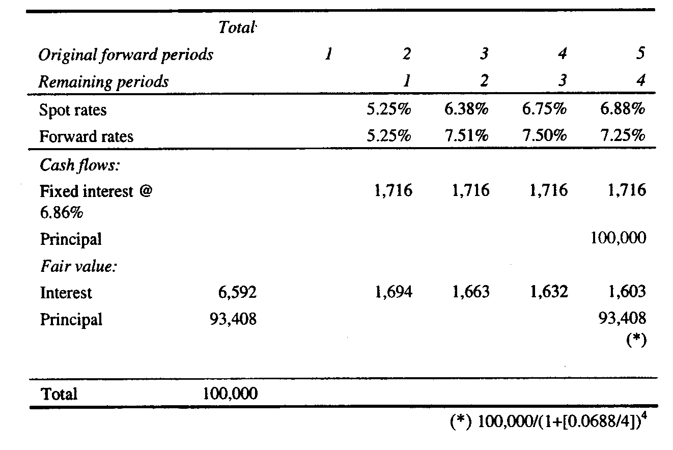
In this example, the enterprise expects to issue a 100,000 one-year debt instrument in three months with quarterly interest payments.  The enterprise is exposed to interest rate increases and would like to eliminate the effect on cash flows of interest rate changes that may occur before the forecasted transaction occurs.  If that risk is eliminated, the enterprise would obtain an interest rate on its debt issuance that is equal to the one-year forward coupon rate currently available in the marketplace in three months. That forward coupon rate, which is different from the forward (spot) rate, is 6.86%, computed from the term structure of interest rates shown above.  It is the market rate of interest that exists at the inception of the hedge, given the terms of the forecasted debt instrument.  It results in the fair value of the debt being equal to par at its issuance.

At the inception of the hedging relationship, the expected cash flows of the debt instrument can be calculated based on the existing term structure of interest rates.  For this purpose, it is assumed that interest rates do not change and that the debt would be issued at 6.86% at the beginning of Period 2.  In this case, the cash flows and fair value of the debt instrument would be as follows at the beginning of Period 2:

Issuance of fixed rate debt
Beginning of period 2 - No rate changes (Spot based on forward rates)

Table #1


Since it is assumed that interest rates do not change, the fair value of the interest and principal amounts equals the par amount of the forecasted transaction.  The fair value amounts are computed based on the spot rates that exist at the inception of the hedge for the applicable periods in which the cash flows would occur had the debt been issued at the date of the forecasted transaction.  They reflect the effect of discounting those cash flows based on the periods that will remain after the debt instrument is issued.  For example, the spot rate of 6.38% is used to discount the interest cash flow that is expected to be paid in Period 3, but it is discounted for only two periods because it will occur two periods after the forecasted transaction occurs.

The forward interest rates are the same as shown previously, since it is assumed that interest rates do not change.  The spot rates are different but they actually have not changed.  They represent the spot rates one period forward and are based on the applicable forward rates.


Hedging instrument

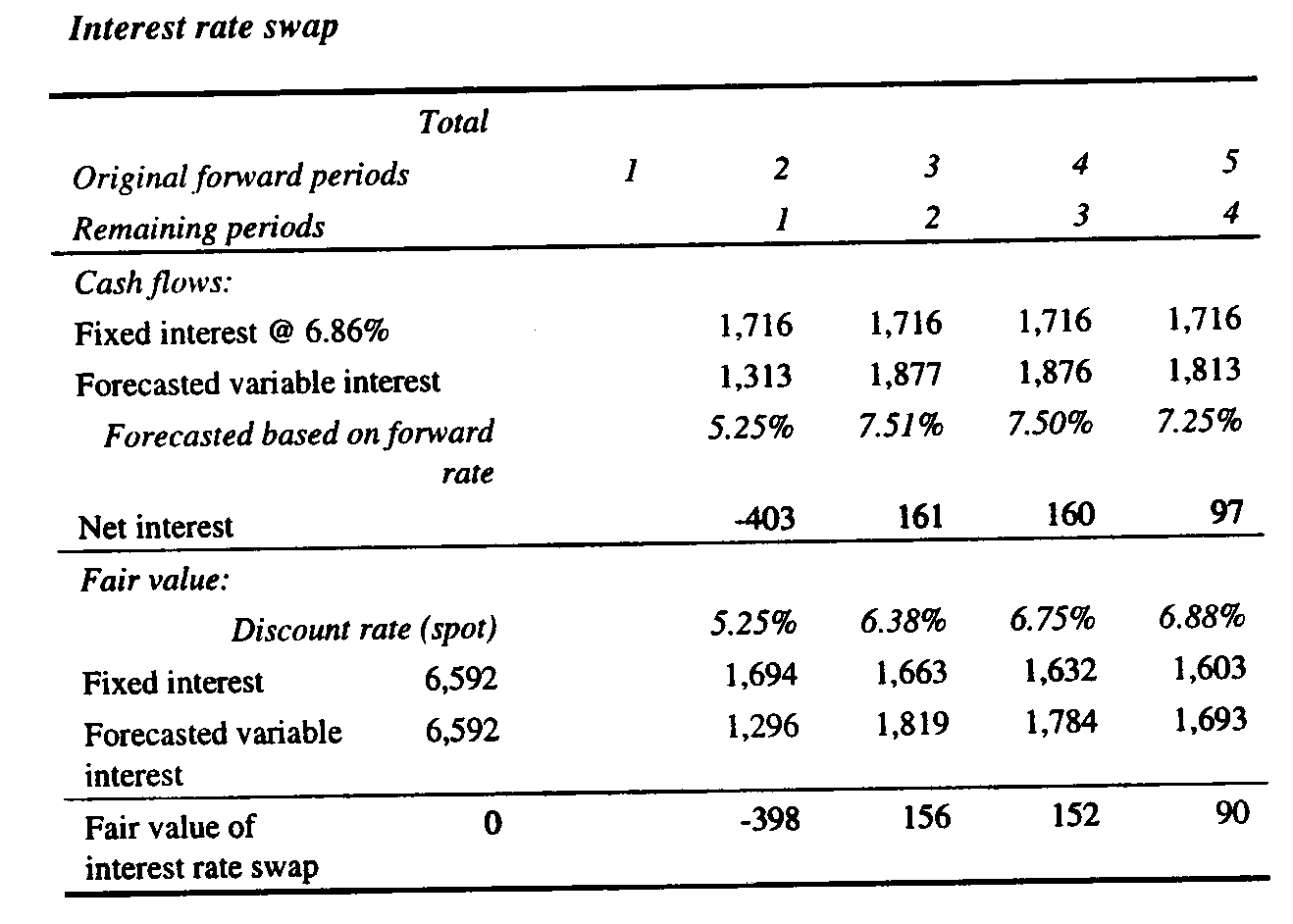
The objective of the hedge is to obtain an overall interest rate on the forecasted transaction and the hedging instrument that is equal to 6.86%, which is the market rate at the inception of the hedge for the period from Period 2 to Period 5.  This objective is accomplished by entering into a forward starting interest rate swap that has a fixed rate of 6.86%.  Based on the term structure of interest rates that exist at the inception of the hedge, the interest rate swap will have such a rate.  At the inception of the hedge, the fair value of the fixed rate payments on the interest rate swap will equal the fair value of the variable rate payments, resulting in the interest rate swap having a fair value of zero.  The expected cash flows of the interest rate swap and the related fair value amounts are shown as follows:

Table #2

At inception of the hedge, the fixed rate on the forward swap is equal to the fixed rate the enterprise would receive if it could issue the debt in three months under terms that exist today.


Measuring hedge effectiveness

If interest rates change during the period the hedge is outstanding, the effectiveness of the hedge can be measured in a number of ways.

Assume that interest rates change as follows immediately prior to the issuance of the debt at the beginning of Period 2:

Yield curve -- Rates increase 200 basis points

Table #3


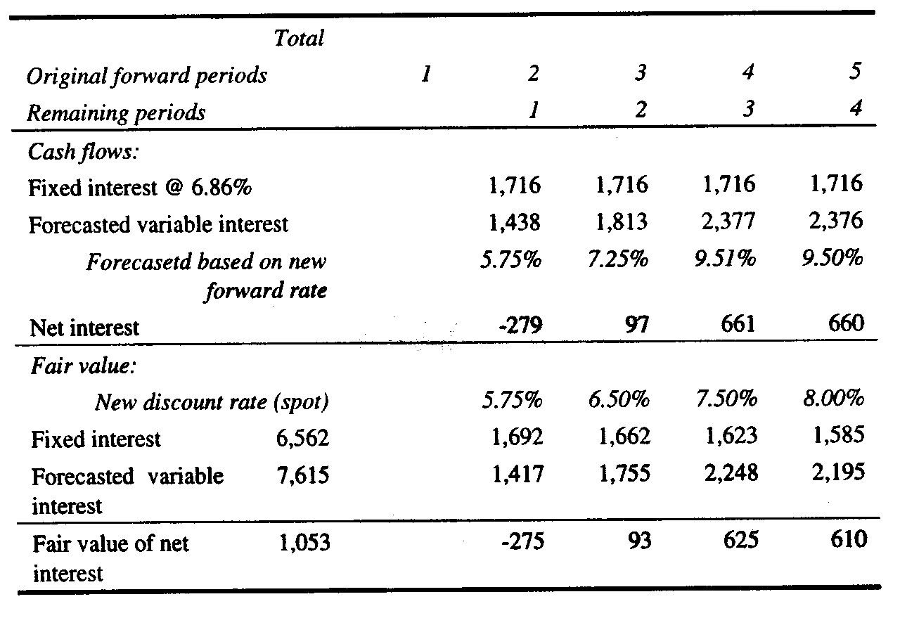
Under the new interest rate environment, the fair value of the pay-fixed at 6.86%, receive-variable interest rate swap which was designated as the hedging instrument would be as follows:

Fair value of interest rate swap

Table #4

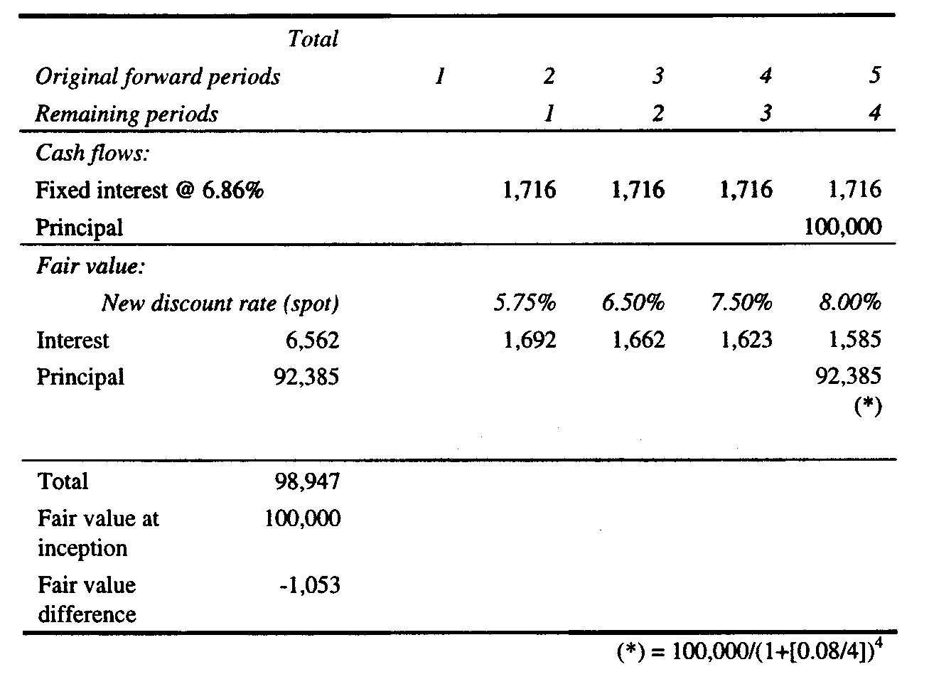
In order to compute the effectiveness of the hedge, it is necessary to measure the change in the present value of the cash flows or the value of the hedged forecasted transaction.  There are at least two methods of accomplishing this measurement.

Method A -- Compute change in fair value of debt

Table #5

Under Method A, a computation is made of the fair value in the new interest rate environment of debt that carries interest that is equal to the coupon interest rate that existed at the inception of the hedging relationship (6.86%).  This fair value is compared with the expected fair value as of the beginning of Period 2 that was calculated based on the term structure of interest rates that existed at the inception of the hedging relationship, as illustrated above, to determine the change in the fair value.  Note that the difference between the change in the fair value of the swap and the change in the expected fair value of the debt exactly offset in this example, since the terms of the swap and the forecasted transaction match each other.

Method B -- Compute change in fair value of cash flows

Table #6

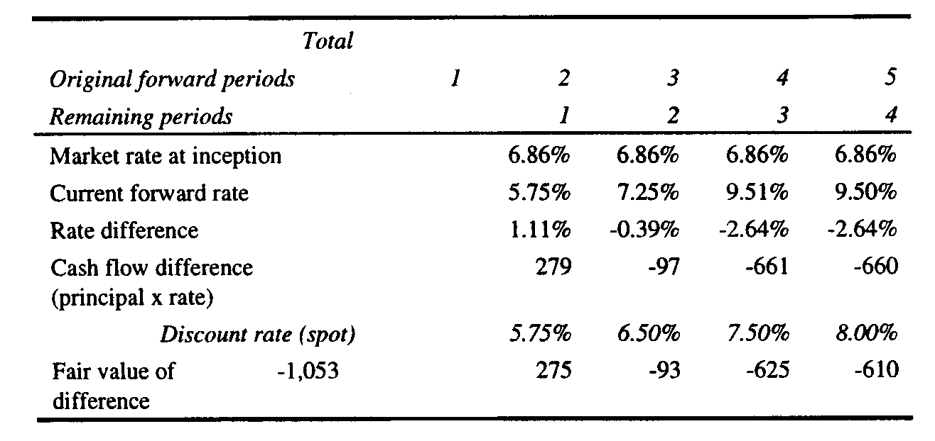
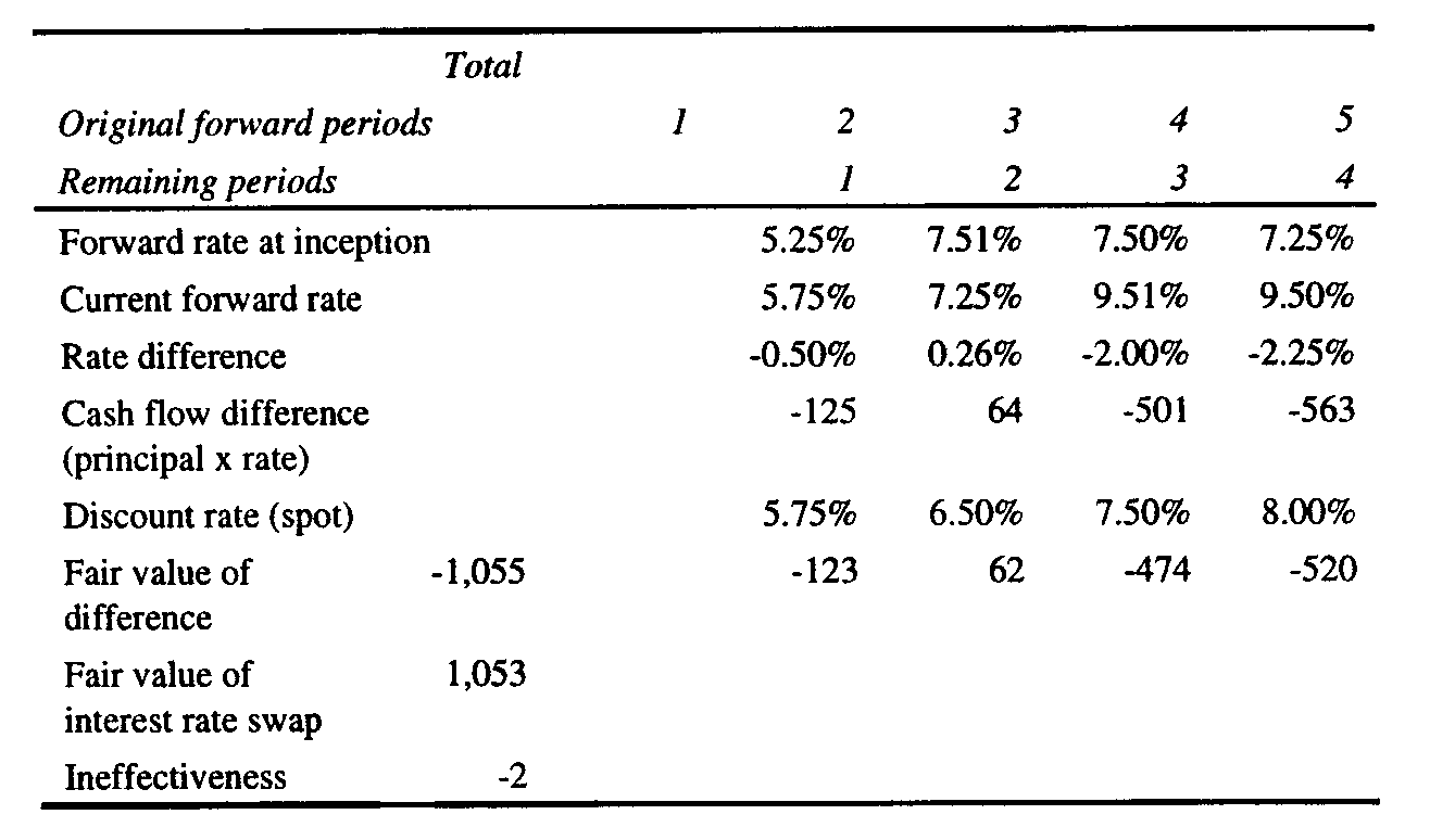
Under Method B, the present value of the change in cash flows is computed based on the difference between the forward interest rates for the applicable periods at the effectiveness measurement date and the interest rate that would have been obtained had the debt been issued at the market rate that existed at the inception of the hedge.  The market rate that existed at the inception of the hedge is the one-year forward coupon rate in three months.  The present value of the change in cash flows is computed based on the current spot rates that exist at the effectiveness measurement date for the applicable periods in which the cash flows are expected to occur.  This method also could be referred to as the "theoretical swap" method (or "hypothetical derivative" method) because the comparison is between the hedged fixed rate on the debt and the current variable rate, which is the same as comparing cash flows on the fixed and variable rate legs of an interest rate swap.

As before, the difference between the change in the fair value of the swap and the change in the present value of the cash flows exactly offset in this example, since the terms match.


Other considerations

There is an additional computation that should be performed to compute ineffectiveness prior to the expected date of the forecasted transaction that has not been considered for purposes of this illustration.  The fair value difference has been determined in each of the illustrations as of the expected date of the forecasted transaction immediately prior to the forecasted transaction, that is, at the beginning of Period 2.  If the assessment of hedge effectiveness is done before the forecasted transaction occurs, the difference should be discounted to the current date to arrive at the actual amount of ineffectiveness.  For example, if the measurement date were one month after the hedging relationship was established and the forecasted transaction is now expected to occur in two months, the amount would have to be discounted for the remaining two months before the forecasted transaction is expected to occur to arrive at the actual fair value.  This step would not be necessary in the examples provided above because there was no ineffectiveness.  Therefore, additional discounting of the amounts, which net to zero, would not have changed the result.

Under Method B, ineffectiveness is computed based on the difference between the forward coupon interest rates for the applicable periods at the effectiveness measurement date and the interest rate that would have been obtained had the debt been issued at the market rate that existed at the inception of the hedge.  Computing the change in cash flows based on the difference between the forward interest rates that existed at the inception of the hedge and the forward rates that exist at the effectiveness measurement date is inappropriate if the objective of the hedge is to establish a single fixed rate for a series of forecasted interest payments.  This objective is met by hedging the exposures with an interest rate swap as illustrated in the above example.  The fixed interest rate on the swap is a blended interest rate composed of the forward rates over the life of the swap.  Unless the yield curve is flat, the comparison between the forward interest rate exposures over the life of the swap and the fixed rate on the swap will produce different cash flows whose fair values are equal only at the inception of the hedging relationship.  This difference is shown in the table below:


Table #7

If the objective of the hedge is to obtain the forward rates that existed at the inception of the hedge, the interest rate swap is ineffective because the swap has a single blended fixed coupon rate that does not offset a series of different forward interest rates.  However, if the objective of the hedge is to obtain the forward coupon rate that existed at the inception of the hedge, the swap is effective, and the comparison based on differences in forward interest rates suggests ineffectiveness when none may exist.  Computing ineffectiveness based on the difference between the forward interest rates that existed at the inception of the hedge and the forward rates that exist at the effectiveness measurement date would be an appropriate measurement of ineffectiveness if the hedging objective is to lock in those forward interest rates.  In that case, the appropriate hedging instrument would be a series of forward contracts each of which matures on a repricing date that corresponds with the occurrence of the forecasted transactions.

It also should be noted that it would be inappropriate to compare only the variable cash flows on the interest rate swap with the interest cash flows in the debt that would be generated by the forward interest rates.  That methodology has the effect of measuring ineffectiveness only on a portion of the derivative, and IAS 39 does not permit the bifurcation of a derivative for purposes of assessing effectiveness in this situation (IAS 39.144).  It is recognized, however, that if the fixed interest rate on the interest rate swap is equal to the fixed rate that would have been obtained on the debt at inception, there will be no ineffectiveness assuming that there are no differences in terms and no change in credit risk or it is not designated in the hedging relationship.


November 23, 2003 message from Ira

Bob,

I've just posted a new article on the Kawaller & Company web site -- "Swap Valuations: The Bank One Swaps Market Precedent". It was published in the latest issue of Risk Magazine, and it was co-authored with John Ensminger and Lou Le Guyader. It may be of particular relevance for those with a tax or regulatory orientation.

If you are interested, you can view it by clicking here: http://www.kawaller.com/pdf/Risk_tax_issues.pdf 

(Or copy this link address and past it into the address field in you internet browser.)

You can also go to the Kawaller & Company website to find the following: " Other articles on derivatives, risk management, and related accounting " A schedule of upcoming conferences relating to these topics; and " A description of Kawaller & Co.'s services

Please feel free to contact me with any questions, comments, or suggestions.

Ira Kawaller Kawaller & Company, LLC   http://www.kawaller.com 

kawaller@kawaller.com  718-694-6270


Casting out on the Internet often results in a catch

Over a year ago I posted a dilemma regarding valuation of interest rate swaps when I attempted to devise a valuation scheme to add to Example 5 in Appendix B of FAS 133 --- http://http://faculty.trinity.edu/rjensen/caseans/133ex05d.htm

On March 24, 2005 I received the following message from a nice man that I do not know named Raphael Keymer [raph@gawab.com]


I think I have a solution to your dilema

I’m responding to a ‘dilema’ you posted on the internet concerning recalculation of example 5 for FAS 133.   I’ve recalculated the example in question on your web page and believe I’ve resolved the difference.


The Jarrow and Turnbill method was not properly implemented

It turns out the implementation of the ‘Jarrow and Turnbill’ methodology was not correct.  When it is properly implemented both valuation methodologies give the same value as the first method employed by you.


Corrections required for Jarrow and Turnbill


Only fixed cash flows on the swap are to be discounted at first

Per the example on pages 435-437, the fixed payments for the swap are considered first, and then only are the floating payments considered.   This is calculated (in the worked example) as the present value of the stream of future fixed cash flows.  The original implementation used a stream of the latest net cash settlement on reset in place of the stream of fixed cash flows.


The present value of the floating cash flows needs to be calculated

The original implementation didn’t calculate the present value of future floating rate cash flows on the swap.


Interpretation of interest rates was inconsistent with Teets & Uhl

Calculation of discount factors is dependant on the interpretation of the time period related to interest rates.  The original Jarrow and Turnbill implementation used interest rates for earlier periods than those used in the Teets & Uhl implementation.  This ‘correction’ will have the least effect on valuation differences.


Revised calculations have been attached in a spreadsheet

I placed his attached spreadsheet at http://www.cs.trinity.edu/~rjensen/133ex05aSupplement.xls

My original Example 5 solution is in the 133ex05a.xls Excel workbook at http://www.cs.trinity.edu/~rjensen/

Also see 133ex05.htm at http://www.cs.trinity.edu/~rjensen/


Return to Bob Jensen's main glossary on derivative financial instruments accounting --- http://http://faculty.trinity.edu/rjensen/acct5341/speakers/133glosf.htm