Bob Jensen's Working Paper 275 on Wolfram Alpha

In 2017 my Website was migrated to the clouds and reduced in size.
Hence some links below are broken.
One thing to try if a “www” link is broken is to substitute “faculty” for “www”
For example a broken link http://faculty.trinity.edu/rjensen/Pictures.htm
can be changed to corrected link http://faculty.trinity.edu/rjensen/Pictures.htm
However in some cases files had to be removed to reduce the size of my Website
Contact me at rjensen@trinity.edu if you really need to file that is missing

Some Things You Might Want to Know About the Wolfram Alpha (WA) Search Engine: The Good and The Evil
as Applied to Learning Curves (Cumulative Average vs. Incremental Unit)
Bob Jensen at Trinity University

Introduction

Wolfram Alpha (WA) Computational Knowledge Search Engine --- http://www.wolframalpha.com/
You may enter a search term (such as "cumulative average") in the search box or a formula (such as "(1000000)(8)^((ln(80/100)/ln(2))"that you want solved.
The search term may be disappointing relative to what you obtain from Google, Bing, or other search engine.
But the formula solving hardly ever disappoints and may even yield very neat publishable formulas, an answer, and a bonus graph of the function.

Wolfram Alpha --- http://en.wikipedia.org/wiki/Wolfram_Alpha

Wolfram Alpha (styled Wolfram|Alpha) is an answer engine developed by Wolfram Research. It is an online service that answers factual queries directly by computing the answer from structured data, rather than providing a list of documents or web pages that might contain the answer as a search engine would. It was announced in March 2009 by Stephen Wolfram, and was released to the public on May 15, 2009.[1] It was voted the greatest computer innovation of 2009 by Popular Science.

Wolfram Alpha for Educators --- http://www.wolframalpha.com/educators/

One evil of WA is that students may enter complex formulas into the search box and receive instant answers (and sometimes graphs) without having to learn much of the analytics that they would otherwise learn by solving formulas in traditional/iterative process that is often valuable in mathematics lessons. Although solutions can be obtained from other software such as Excel, WA is more of a one-step process that takes much of the drudgery and learning process that comes even with the other software. WA presents problems similar to and well beyond the issue of whether to allow graphing calculators.

But WA need not be so evil if instructors simply control when and if students are allowed to use WA, such as by not allowing WA to be used on examinations. That could motivate students to learn how to solve formulas without the aid of WA as well as to use WA to early on better understand functions before taking examinations.

I am awestruck by the good features of WA for ease of computation, preparing papers for publication, and for better understanding complicated formulas.

Although I knew the general features of WA, this week I seriously used it when confronted with some formulas I needed to solve.

My SJM Paper

"Reconciliation of Learning Rates Between the Cumulative Average Versus Incremental Learning Rate Models," by Robert E. Jensen, Scandinavian Journal of Management, Vol. 7, No. 2, 1991, 137-142 ---
http://www.cs.trinity.edu/~rjensen/temp/WorkingPaper275.pdf

After nearly 20 years I completely forgot about this paper that I drafted in 1989. In 1989 I did not own a PC. Being an old teacher of FORTRAN and COBAL, I could've written a main frame computer program to solve the formulas in the SJM paper, but at the time Trinity University was having troubles with its main frame computer, and I did not own or use a PC until I purchased a PC in 1990. In 1989 I spent days on an HP memory calculator solving the formulas in Table 1 of the paper. The problem was not so much solving the formulas as it was iteratively finding the parameters that equated the cumulative average versus incremental unit learning models.

Out of the blue on September 14, 2010 I received a message from a very polite Australian professor named Chris Deeley who challenged the computations in my SJM paper published in 1991. My initial reaction was that he was probably correct since I'd never subsequently verified my 1989 HP calculator solutions with any modern software like Excel. Subsequently, I think I have verified the numbers in the paper by using Excel. However, just for the heck of it I also verified some of the key numbers using Wolfram Alpha (WA). I'm truly impressed with some of the things WA will generate that cannot be generated in Excel.

In my particular circumstances the Goal Seek utility in Excel saved hours of tedious computations on a calculator ---
http://office.microsoft.com/en-gb/excel-help/about-goal-seek-HP005203894.aspx

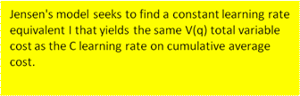
It turned out that both Jensen and Deeley computed their numbers correctly under their different models. Professor Deeley defined a somewhat different incremental learning rate model. Deeley assumes the I(j,q) learning rate varies when computing each marginal unit cost whereas Jensen assumes the I(q) marginal unit cost varies only with the number of units, q, produced in total and the total variable cost V(q)..

Hence comparing Deeley versus Jensen outcomes is like comparing apples and oranges, although they do get the same total variable cost. It's just that the patterns of marginal unit costs differ in arriving at total variable cost. It came to my great relief that the numbers that I computed on a calculator in 1989 held up in 2010 under both Excel and Wolfram Alpha.

Consider the following numbers for q=8 units of product and an incremental learning rate of 80% which means that the u(q) marginal per unit of product will be 80% each time q is doubled. This 80% learning curve in the aircraft production industry was shown by Theodore Paul Wright to be somewhat like the inexplicable Moore's Law is to the cost of computer memory. Both inexplicably hold true under different circumstances.

Suppose the marginal cost of the first unit is u(1)=$1,000,000.

Here are examples of three test numbers that I first checked in Excel for Jensen's 1989 model on Page 140 of the SJM paper:

-0.321928 = i exponent of the 80% learning rate
$512,000 = u(8) marginal cost of Unit 8
$5,345,914 = V(8,80) cumulative variable cost of the first eight production units (e.g., airplanes)

The WA code formulas that I first used to test these calculations in Wolfram Alpha are as follows:

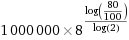
-0.321928 = i = (ln(80/100))/(ln(2)) where ln( ) is a natural base e logarithm.
$512,000 = u(8) = 1000000*(8^(( ln(80/100))/(ln(2)))
$5,345,914 = V(8,80)= (1000000)Sum(j=1,8,j^(ln(80/100)/ln(2))) This WA code did not work in Excel

Wolfram Alpha Extensions

I derived the three numbers above easily in Excel, although in Excel I simply computed V(8,80) as the sum of u(1) thru u(8). Now comes the interesting part. Suppose that I was writing a paper and wanted to publish the three functions shown above. In code, these functions are very difficult for readers of a paper. However, when these codes are read into WA all sorts of neat things happen. If I wanted to publish these results or better explain to students what is being calculated, I could cut and paste the WA math interpretations generated by the incomprehensible code.

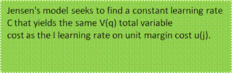
Firstly, I get Wolfram Alpha formatted formulas that I can cut and past into a paper.

-0.321928 = i = (ln(80/100))/(ln(2))

                        =   where log is a natural logarithm

$512,000 = u(8) = 1000000*(8^(( ln(80/100))/(ln(2)))

                        = where log is a natural logarithm

$5,345,914 = V(8,80 = (1000000)Sum(j=1,8,j^(ln(80/100)/ln(2)))

                        =    where log is a natural logarithm

Secondly, I get some added WA information for extending the formulas to the limit in a continuum:

=

Thirdly for some functions, graphs and other information about those functions will be generated (including regressions and probability distribution graphs)
http://www.wolframalpha.com/examples/

A few other things to try in Wolfram Alpha:

Excel Solutions and Extensions of SJM Paper

Excel is still more useful than WA for repetitive calculations. As mentioned above, the huge time saver in this instance is the Goal Seek utility in Excel.
The Excel verifications of the numbers in my SJM paper and some extensions are shown below:

Equivalent C =

87.43

From Goal Seek

Fixed I =

The 87.43% learning rate agrees with C(80,8) on Page 140 of the paper

-0.1938545

-0.321928095

The i= -0.321928 exponent appears on Page 140 of the paper

u(1)=

$1,000,000

u(1)=

$1,000,000

u(8)=

$545,574

u(8)=

$512,000

The u(8) = $512,000 cost of the 8th unit agrees with Page 140 of the paper

Marginal

Variable

Cumulative

Double j

Marginal

Variable

Cumulative

Double j

Cost

Average

Learning

Cost

Average

Learning

u(j)

V(j)

v(j)

Rate

u(j)

V(j)

v(j)

Rate

1000000

748534

1748534

874267

0.8743

800000

1800000

900000

0.8000

676005

2424539

808180

702104

2502104

834035

632831

3057370

764342

0.8743

640000

3142104

785526

0.8000

602550

3659920

731984

595637

3737741

747548

579468

4239388

706565

0.8743

561683

4299424

716571

0.8000

560952

4800340

685763

534490

4833914

690559

545574

5345914

668239

0.8743

512000

5345914

668239

0.8000

V(8)=

$5,345,914

=Sum

From Goal Seek

$5,345,914

=Sum = V(8)

This V(8) total variable cost agrees with Page 140 of the paper

$668,239

=Average

$668,239

=Average

This average is incorrectly given as $664,489 on Page 140 of the paper

Fixed C =

Equivalent I =

67.79

From Goal Seek

-0.3219281

-0.560926783

u(1)=

$1,000,000

u(1)=

$1,000,000

u(8)=

$354,573

u(8)=

$311,482

Marginal

Variable

Cumulative

Double j

Marginal

Variable

Cumulative

Double j

Cost

Average

Learning

Cost

Average

Learning

u(j)

V(j)

v(j)

Rate

u(j)

V(j)

v(j)

Rate

1000000

600000

1600000

800000

0.8000

677867

1677867

838933

0.6779

506311

2106311

702104

539970

2217837

739279

453689

2560000

640000

0.8000

459503

2677340

669335

0.6779

418187

2978187

595637

405442

3082782

616556

391911

3370098

561683

0.8000

366028

3448810

574802

0.6779

371329

3741427

534490

335708

3784518

540645

354573

4096000

512000

0.8000

311482

4096000

512000

0.6779

Both models are fairly close in marginal cost outcomes (Jensen in red, Deeley in blue) for q=8.
They will converge as q increases.

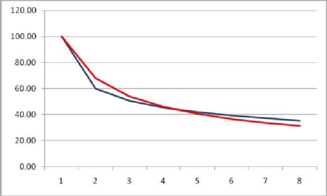
In my opinion, both the Jensen and Deeley models have a learning rate that is too high between the u(1) marginal cost of the first unit vis-à-vis the marginal cost u(2) of the second unit.

Two online spreadsheets are available at
http://www.cs.trinity.edu/~rjensen/temp/WP275Table02b.xlsx
http://www.cs.trinity.edu/~rjensen/temp/WP275Table03b.xlsx

Having verified the main numbers that appear in the Table 1 of my 1991 SJM paper, I did find a few corrections.

On Page 138, the c in Equation 3 should've been upper case.

On Page 140, ln (0.80/100) should read ln (80)/100))

On Pages 140 and 141, $664,489 should read $668,239

Updates

September 22, 2010 message from Deeley, Chris [CDeeley@csu.edu.au]

Bob

I have now solved the riddle (as you already had) of why our two sets of numbers differ. Mine bases parity on incremental cost, while your's bases parity on total cost (and also, of course, cumulative average cost). This point is made perfectly clear below Table 1 where you refer to “what cumulative average model learning rate would achieve the same total cost”. I must have overlooked this earlier and mistakenly assumed that you were trying to establish parity with respect to incremental cost.

I suggest a sensible synthesis is to acknowledge that we have closed-form equations for (1) converting incremental rates into cumulative average rates if parity is with reference to cumulative average costs, and (2) converting cumulative average rates into incremental rates if parity is with reference to incremental costs. That being the case, I don’t see why Table 1 cannot be constructed on that basis. I assume the main objective of the exercise is to determine which curve is more realistic (to date) and therefore presumed to be the more reliable for forecasting purposes. It doesn’t really matter what the points of parity and comparison are, so long as they are clearly identified.

Anyway, I’ll carry on with my table and send you the finished product. I suspect that the “hybrid” table will not take long to complete.

Chris

Chris Deeley

Senior Lecturer in Accounting & Finance

School of Accounting, Faculty of Business

Charles Sturt University, Locked Mail Bag 588

Wagga Wagga, NSW 2678

Ph: +612 69332694 Fax: +612 69332790

September 23, 2010 message from Deeley, Chris [CDeeley@csu.edu.au]

Bob

Thanks for this. I must say I find the material you’ve made available on the Internet most fascinating, especially the comments on retirement, which is a key interest of mine. In Australia one cannot be forced to retire because of age. I’m 66 and not planning to retire anytime soon. I switched out of a defined benefit pension scheme and into a defined contribution scheme some time ago, so I have a financial incentive to stay on a payroll. Fortunately my wife is on an indexed pension, so we have a good safety net.

I’ve now completed my “hybrid” table, which establishes parity between the two learning curves with respect to (1) cumulative average cost when the incremental learning rate is held constant, and (2) incremental cost when the cumulative average learning rate is held constant. This avoids the issue of non-closed-form algebraic solutions, as mentioned in your SJM article (although a suitable solution algorithm, if there is one, would overcome that problem). Unfortunately, I still struggle to compute accumulated costs from a given incremental learning rate for values of q above 200 (assuming that we start with q = 1). This explains the question marks in my table, which you may be able to quantify for me using Wolfram Alpha (if you have the time and inclination). You’ll see that the equivalency figures in the left-hand part of my table are identical to yours, which comes as no surprise after eliminating the apples v oranges element.

Re worthwhile retirement activities: how about reviewing submitted papers for journals/conferences? Maybe you already do this? I also find trading shares is a fascinating pastime.

My own research interests are mainly theoretical. It’s amazing how much stuff is out there which is wrong, but so difficult to change. For example, I contend that the conventional approach to solving general annuity problems is invalid when the frequency of payments exceeds the frequency of interest compounding. I’ll attach a draft paper on this topic, in case it may be of interest.

I hope I haven’t taken up too much of your time.

Chris

Table II. Reconciliation of incremental & cumulative average learning curves
				Incremental learning rate:	80%				Cumulative average learning rate:	80%
			Cumulative average learning					Incremental learning
	Cumulative			rate			Incremental			rate
	average cost parity		varies			cost parity			varies
q	U	CAC	C %	U	CAC	CAC	U	I %	CAC	U
1	1,000,000	1,000,000		1,000,000	1,000,000	1,000,000	1,000,000		1,000,000	1,000,000
2	800,000	900,000	90.000	800,000	900,000	800,000	600,000	60.000	800,000	600,000
3	702,104	834,035	89.181	718,482	834,035	702,104	506,311	65.089	719,067	506,311
4	640,000	785,526	88.630	664,465	785,526	640,000	453,689	67.356	665,450	453,689
5	595,637	747,548	88.223	624,457	747,548	595,637	418,187	68.696	625,713	418,187
6	561,683	716,571	87.904	592,982	716,571	561,683	391,911	69.602	594,426	391,911
7	534,490	690,559	87.644	567,232	690,559	534,490	371,329	70.266	568,811	371,329
8	512,000	668,239	87.427	545,574	668,239	512,000	354,573	70.779	547,251	354,573
9	492,950	648,763	87.241	526,974	648,763	492,950	340,546	71.190	528,724	340,546

10	476,510	631,537	86.062	481,203	607,357	476,510	328,552	71.529	508,707	328,552
20	381,208	524,247	86.121	413,497	524,247	381,208	260,614	73.261	415,429	260,614
30	334,559	467,330	85.639	364,177	467,330	334,559	228,091	73.992	366,044	228,091
40	304,966	429,836	85.329	332,409	429,836	304,966	207,631	74.425	334,190	207,631
50	283,827	402,434	85.106	309,523	402,434	283,827	193,080	74.721	311,222	193,080
60	267,647	381,130	84.933	291,913	381,130	267,647	181,975	74.942	293,538	181,975
70	254,690	363,869	84.794	277,757	363,869	254,690	173,097	75.115	279,317	173,097
80	243,973	349,465	84.679	266,021	349,465	243,973	165,766	75.256	267,521	165,766
90	234,895	337,176	84.581	256,059	337,176	234,895	159,562	75.374	257,508	159,562

100	227,062	326,508	84.496	247,451	326,508	227,062	154,213	75.474	248,852	154,213
200	181,649	263,600	83.994	197,389	263,600	181,649	123,271	76.044	198,487	123,271
300	159,421	232,211	83.741	172,841	232,211	159,421	108,157	76.316	?	108,157
400	145,319	212,122	83.578	157,275	212,122	145,319	98,577	76.488	?	98,577
500	135,246	197,694	83.460	146,166	197,694	135,246	91,736	76.610	?	91,736

1bn*	1,267	?	?	?	?	1,267	859	78.967		859
* Total costs in $million
q = units of accumulated prd'n					U = Incremental unit cost					CAC = cumulative average cost

******************

Chris also seen me his latest working paper on an entirely different topic.

September 23, 2010 message from Chris Deeley cdeeley@csu.edu.au

Bob
Yes, by all means post my working paper on general annuities on the AECM website. I suspect that Wolfram Alpha may not be able to handle this sort of thing. In fact, I wouldn’t be surprised if the application of standard maths has created and entrenched the error. Chris

Chris Deeley
Senior Lecturer in Accounting & Finance
School of Accounting,
Faculty of Business
Charles Sturt University,
Locked Mail Bag 588
Wagga Wagga, NSW 2678
Ph: +612 69332694 Fax: +612 69332790
Email: cdeeley@csu.edu.au
Web: www.csu.edu.au

I put his paper on one of my Web servers. I'm sure that Chris will appreciate any comments that you have regarding this technical topic. It may be a good exercise for accounting and finance students to study this paper.

"IDENTIFICATION AND CORRECTION OF A COMMON ERROR IN GENERAL ANNUITY CALCULATIONS," by Chris Deeley, Charles Sturt University, Australia., September 23, 2010 Working Draft ---
http://www.cs.trinity.edu/~rjensen/temp/DeeleyAnnuityCorrections.pdf

Chris Deeley in Australia and I have been corresponding regarding an antique learning curve paper that I published nearly 20 years ago. You can read some of our correspondence at http://faculty.trinity.edu/rjensen/theorylearningcurves.htm
In that correspondence I discuss the good and evil of the Wolfram Alpha computational search engine.

Instructors might want to consider adding this to their teaching modules on time value of money and annuity mathematics of finance.

Working Paper 440
Annuities With Unequal Compounding and Payment Periods: The CFA Deconstruction Analysis
Bob Jensen at Trinity University

Financial calculators and Excel financial formulas for computing present value, interim payments, and rates of return assume that p=m where p is the number of equally-spaced payments per year and m is the number equally-spaced interest compoundings per year. Complications introduced by p not being equal to m are not trivial problems. These complications are overlooked in many (probably almost all) mathematics of finance modules in both high school and college courses.

This note will demonstrate how to deal with complications when the number of payments per year is unequal to the number in times interest is compounded per year. This is not a purely academic problem. Companies buying and selling annuities often do not want to change the number of times interest is compounded every time they change the number of payments per year in a contract such as semi-annual payments versus quarterly payments versus monthly payments.

The paper was inspired by the following working paper sent to me by an Australian professor named Chris Deeley. Chris subsequently allowed me to put his paper on one of my Web servers:

"IDENTIFICATION AND CORRECTION OF A COMMON ERROR IN GENERAL ANNUITY CALCULATIONS"
by Chris Deeley cdeeley@csu.edu.au
Working Paper, Charles Sturt University, Australia, September 22, 2010
http://www.cs.trinity.edu/~rjensen/temp/DeeleyAnnuityCorrections.pdf

For illustrative purposes I will focus on the following example on Page 11 of Professor Deeley's working paper:

Example 2
A loan of $1million is to be repaid in equal monthly installments over four years. If the annual interest rate is 10% compounded semi-annually, how much is the monthly repayment?

The two solutions given by Professor Deeley for p=12 payments per year and m=2 interest compoundings per year are as follows:

Deeley Solution 1 PMT = $25,265.60 per month which Professor Deeley claims the "conventional solution"

Deeley Solution 2 PMT = $25,260.70 per month which Professor Deeley claims is his "proposed better solution"

I contend that there is a CFA Deconstruction and Rate Equivalence solution that I offer as an "alternate conventional solution" used of Certified Financial Analyst (CFA) examinations.

CFA Deconstruction PMT = $25,483 per month which conforms to David Frick's solution tutorial

I show how to calculate this $25,483 using both Wolfram Alpha and Excel in my Working Paper 440 ---
Bob Jensen's analysis of Annuities With Unequal Compounding and Payment Periods: The CFA Deconstruction Analysis
http://faculty.trinity.edu/rjensen/TheoryAnnuity01.htm

July 31, 2012 message from David Albrecht

I'm sharing the link to my cost accounting syllabus for a couple of reasons.
http://profalbrecht.wordpress.com/2012/07/31/my-cost-accounting-syllabus/

First, it shows what leading educators say should be in a syllabus. Second, I've spent a lot of time making it pleasing to the eyes.

Dave Albrecht

Hi David,

This is a good start, and I commend you for the effort.

You should add a link to MAAW's great cost accounting modules ---
http://maaw.info/JITMain.htm

For example, one module you might want to add in such a syllabus is "Lean Accounting" ---
http://maaw.info/JITMain.htm

Personally, I would probably play down 80% learning curves since the early work on learning curves in airplane manufacturing really don't extrapolate well to most other industries ---
http://faculty.trinity.edu/rjensen/theorylearningcurves.htm

You can, however, bring in more recent evidence on learning curves.

"Ethanol learning Curve—the Brazilian experience," by José Goldemberga, Suani Teixeira Coelhob, Plinio Mário Nastaric, Oswaldo Lucond, Biomass and Bioenergy, Volume 26, Issue 3, March 2004, Pages 301–304

Abstract

Economic competitiveness is a very frequent argument against renewable energy (RE). This paper demonstrates, through the Brazilian experience with ethanol, that economies of scale and technological advances lead to increased competitiveness of this renewable alternative, reducing the gap with conventional fossil fuels.

Jensen Comment
Unlike corn ethanol, sugar cane ethanol is a viable renewable energy alternative. Corn ethanol, however, just does not get enough energy out for the energy going into its refining. Corn ethanol can only survive on the basis of government subsidies and tariff. If we want ethanol in our fuel, we should shift to cane sugar ethanol production and importing rather than raise tariff barriers against cane sugar ethanol imports.

There is quite a lot of learning curve literature in the energy field. For example, look at
http://www.sciencedirect.com/science/article/pii/S0301421505001795

Abstract

The extent and timing of cost-reducing improvements in low-carbon energy systems are important sources of uncertainty in future levels of greenhouse-gas emissions. Models that assess the costs of climate change mitigation policy, and energy policy in general, rely heavily on learningcurves to include technology dynamics. Historically, no energy technology has changed more dramatically than photovoltaics (PV), the cost of which has declined by a factor of nearly 100 since the 1950s. Which changes were most important in accounting for the cost reductions that have occurred over the past three decades? Are these results consistent with the notion that learning from experience drove technical change? In this paper, empirical data are assembled to populate a simple model identifying the most important factors affecting the cost of PV. The results indicate that learning from experience, the theoretical mechanism used to explain learning curves, only weakly explains change in the most important factors—plant size, module efficiency, and the cost of silicon. Ways in which the consideration of a broader set of influences, such as technical barriers, industry structure, and characteristics of demand, might be used to inform energy technology policy are discussed.