|
Chapter 6
All the real knowledge which we possess,
depends on methods by which we distinguish the similar from the
dissimilar. The greater number of natural distinctions this method
comprehends, the clearer becomes our idea of things. The more numerous the
objects which employ our attention the more difficult it becomes to form such a
method and the more necessary.
For we must not join in the same genus the
horse and the swine, tho' both species had been one hoof'd nor separate in
different genera the goat, the reindeer and the elk, tho' they differ in the
form of their horns. We ought therefore by attentive and diligent
observation to determine the limits of the genera, since they cannot be
determined a priori. This is the great work, the important labour, for
should the Genera be confused, all would be confusion.
[Carolus Linaeus, Swedish Botonist, Genera Plantarum, 1739]
General observations drawn from particulars
are the jewels of knowledge, comprehending great store in a little room.
[John Locke, 17th Century British Philosopher]
Science is built up with facts, as a house is
with stones. But a collection of facts is no more a science than a heap of
stones is a house.
[Jules Henri Poincare, French Mathematician, La
Science et l'Hypothese, 1908]
Throughout the history of the development of
scientific method the only lasting theories have been those that began with good
observation, with noting peculiar relations among measurements, or with firm
groundwork of classificatory, taxonomic, and clinical experience. In those
cases where theory appears to have preceded observation, it will often be found
that the theory that preceded measurement is the same as the post-measurement
theory in name only.
[Raymond B. Cattell, Research Professor in
Psychology at the University of Illinois (Urbana), in Personality and
Motivation Structure and Measurement (New York: World Book Company, 1957, p.
3)]
Comparing mills is like comparing apples and
oranges. No two are identical and the local environmental problems and
priorities are different.
[J. L. McClintock, Weyerhaeuser Corporation,
as quoted in Paper Profits: Pollution in the Pulp and Paper Industry (New
York: Council on Economic Priorities, 1971)]
One picture is worth more than ten thousand
words.
[Anonymous Chinese Proverb]
In thy face I see
The map of honor, truth, and loyalty.
[Shakespeare, Henri VI]
His face is the worst thing
about him.
[Shakespeare, Measure for Measure]
When men are calling names and making faces,
And all the world's ajangle and ajar,
I meditate on interstellar spaces
And smoke a mild seegar.
[Burt Leston Taylor, 19th
Century Poet, Canopus]
6.1--Introduction
The purpose of this chapter is largely to
consider a number of approaches in taxonomy and the quest for empirical
types. The approaches discussed later on in this chapter are those which
either (i) result in sensory displays (confined here to visual displays)
enabling human observers to search for "types" in a subjective manner,
or (ii) result in mathematical partitionings of entities into "types"
via numerical taxonomy techniques. The analysis may consist of more than
merely searching for types on the basis of multivariate corporate social impacts
such as those illustrated in Appendix A. A point made repeatedly in
earlier chapters is that corporate social accountings will typically yield
masses of data, some of which are qualitative and some of which are quantitative
but measured in differing units (percentages, man-hours, tons, cubic yards,
dollars, etc.). In such situations some type of parsimony is needed for
both reporting and analyzing such a hodgepodge of disconnected facts.
The accustomed accounting procedure of converting everything to monetary units
and then aggregating by arithmetic methods (usually addition) to achieve
parsimony in social accounting is fraught with difficulties. The usual
statistical multivariate data analysis techniques (e.g., multiple regression,
discriminant, factor and variance analyses) are somewhat more flexible, but
frequently suffer from overly restrictive assumptions and/or difficulties in
interpretation.
The major purpose of Chapter 6 is to explore some
more general techniques for condensing and evaluating multivariate quantitative
data, although some of the techniques may also accommodate qualitative
differences. In an effort to avoid being too abstract, such techniques are
applied to a number of social accounting variables observed on twelve electric
utility companies. Particular emphasis is placed upon graphic and other
visual display techniques under varying circumstances. Several important
data transformations and numerical taxonomy are also examined.
6.2--Theory of Types
Raymond Cattell, authority of personality
typology, once stated:
...The Experience of science is that a tidy taxonomy is never
useless, but full of systematic profits for research. For example, in many
social psychological problems, in which one person is the stimulus situation for
the behavior of another, perceptions depend on type affiliations. Types
are thus not just unnecessary intermediate concepts--not just another instance
of academic punditry or compulsion--but, if properly conceived, necessary and
economical operational concepts...1
The term "type" has intuitive meaning
to nearly everyone, although forming a precise definition (along with related
concepts such as group, pattern, cluster, configuration, factor, genus, species,
etc.) is difficult.2 Entities classified as a type
supposedly are "more alike" in terms of certain properties than other
entities not of that type. Different properties (attributes, traits, etc.)
may give rise to different groupings of entities into types. In addition,
what constitutes a "type" depends on the basis for defining similarity
(association, distance, affinity, interaction, etc.) and precise constraints
imposed by the definition of what constitutes or does not constitute a
"type." For example, "types" may be mutually exclusive
versus intersecting, collectively exhaustive versus selective,
discrete partitions versus having gradations of belongedness, and so on.
Ball lists seven uses of cluster analysis which
apply to the quest for types in general:
-
Finding a true typology;
-
Model fitting;
-
Prediction based on groups;
-
Hypothesis testing;
-
Data exploration;
-
Hypothesis testing;
-
Data reduction.3
These are not necessarily mutually exclusive, and
prediction seemingly may arise under any of the above purposes. Cattell
writes:
Briefly to indicate what this second step may comprise, one
should point out that Aristotelian classification permits one to make
predictions of the kind: "This is a dog; therefore it may bite";
"This is a schizophrenic; therefore the prospect of remissions is not
high." In other words, a classification of objects by variables of
one kind may permit prediction on others not at the time included.
Parenthetically, despite the illustrations, these predictions need not be
categorical, but can be parametric.4
I do not pretend to be the first to suggest that
business firms might be typed. For many years business firms have been
viewed according to industry types, size classifications, production or
marketing regions, capital intensity, labor intensity, etc. I am
suggesting, however, that researchers devote more attention to classifying
business firms into empirical types on the basis of social impacts. In
the next chapter (Chapter 7) some attention is devoted to classifying firms or
persons on the basis of human perceptions. In this chapter (Chapter 6) our
concern will be more upon classifications based upon general statistics on
businesses, e.g., earnings margins, product prices, pollution expenditures,
etc. Research along similar lines has taken place with respect to finding
nation types. Rummell, for example, writes:
Students of comparative relations have always dealt with
nation types. One type that has played a dominat role in the theoretical
and applied international relations is that of the powerful nation. This
type has become so widely recognized as implying set characteristics and
international behavior that we readily employ the noun "powers" alone
to refer to nations of this kind. Such nation "types" as
"modern," underdeveloped," "Constitutional,"
"status quo nations," "prismatic," "aggressive,"
"traditional," and "nationalistic," have only to be
mentioned to evidence the prevalence of typal distinctions.
The problem with the prevailing types is that the rationale
underlying the categorization is not explicit (and that it is not clear whether
the type really divides different kinds of variance). If we are to deal in
types, a clear and empirical basis for the distinctions must be made.5
1
R. B. Cattell, Personality and Motivation Structure and Measurement
(Yonkers-on-Hudson, New York: World Book Company, 1957, p. 383).
2 Definition
varieties for "type" are discussed by Cattell, Ibid, pp.
364-69.
3 G. H. Ball,
Classification Analysis, Stanford Research Institute, Project 5533, Stanford,
California, 1971.
4 R. B.
Cattell,
"Taxonomic Principles for Locating and Using Types (and the Derived Taxonome Computer Program)," in Formal Representation of Human Judgment,
Edited by B. Kleinmuntz (New York: John Wiley & Sons, Inc., 1968, p. 104).
5 R. J.
Rummell, The Dimensions of Nations (Beverly Hills, California: Sage
Publications, 1972, p. 300).
6.3--Condensation of Data: The Need for
Parsimony
In spite of the difficulties of detecting,
recording, and attestation of corporate impact data, equally difficult problems
arise in utilizing such data. Decisions are made by humans (or decision
rules set by humans) and, unfortunately, the human mind is easily boggled by
relatively small amounts of data. As facts and figures begin to pile up,
the decision maker devises means of organizing, categorizing, and summarizing in
an effort to achieve parsimony in what he or she must comprehend and
evaluate. At one end of the spectrum are masses of disconnected facts; at
the other end are a few condensed statements or measures.
Within a firm, the degree of condensation of
traditional accounting data varies with the manager's level in the organization
and the use to which information is to be put. In social accounting we are
still at a stage where we have a basket of apples, oranges, rocks, carrots,
thistles, roses, rabbits, turtles, monkeys and ad infinitum.
Methods of condensation of heterogeneous social accounting items are
undeveloped.
In traditional accounting, condensation typically
consists of additive aggregation, e.g., operating managers may only see
labor cost aggregated over people and time. Top management examines
summary reports over multiple divisions, subsidiary companies, and longer
intervals of time. The investing public receives even more parsimonious
aggregations.
Another means of data condensation is the filtering
process. For example, budget or standard items may automatically be
compared (by computer) with actual out comes. Operating managers may only
act upon "exception" phenomena, e.g., aberrant phenomena which vary
from standard by some predetermined amount. The aberrant phenomena are
"filtered" out and acted upon. Similarly, public press releases
are usually about aberrant events apart from routine day-to-day happenings.
Typically an analysis is conducted
whenever hidden or obscure relationships are suspected which are not evident in
either the basic or aggregated data. Analysis may, in turn, facilitate
further condensation and parsimony, especially if the analysis yields crucial
"measurements" needed to achieve further condensation. The term
"analysis" has a connotation of breaking something down into component
parts, whereas "condense" implies combining component parts into a
denser whole. However, in science the term "analysis" does not
necessarily imply less parsimony, e.g., one of the objectives of factor
"analysis," component "analysis," cluster
"analysis," regression "analysis," and other statistical
analysis tools may be that of achieving parsimony. As such, some form of
"analysis" may be part of a data condensation process.
Similarly, in accounting a cost analysis may entail decomposition of "total
cost" into various "component costs." However, this is not
necessarily the same as moving a step backwards on the condensation
spectrum. For example, total cost may be analyzed to break it down into
fixed and variable components. The analysis may utilize detailed data from
labor and materials records, but the analysis may identify a relationship (e.g.,
linear) which facilitates parsimony and condensation.
In corporate financial accounting, the
higher-most levels of condensation (after much aggregation, filtering, and
analysis) are financial statements items and various computed statistics (e.g.,
working capital ratios and earnings-per-share) derived from financial statement
items. For example, the total assets reported (in billions of dollars) at
the bottom of a General Motors Corporation annual report is a condensed measure
of the millions of heterogeneous items of value held by the company. The
condensation process which yielded such a figure for G. M. Assets entailed a
myriad of accounting "rules" of measurement.
At nearly every point in the accounting
condensation process, accountants disagree as to the proper
"rule." As the condensations become more parsimonious, the
accounting disputes are more pronounced. One of the constant sources of
difficulty is the penchant (based on centuries of tradition) of condensing on
the basis of monetary units (i.e., a numeraire). For example, cash in bank
accounts, inventories, land, buildings, and all other items termed "assets"
in the General Motors balance sheet are measured in dollars, which in turn,
makes the heterogeneous items additive in a common scale of measurement.
Since it is even more difficult to measure most
corporate social impacts in monetary units, accountants are reluctant to extend
financial boundaries into unexplored social accounting territory. Attempts
to do so (e.g., the Abt Associates Social Audits6) have been
highly controversial both as to method and to purpose. Social audits have
primarily been confined to descriptive listings of corporate social endeavors,
with little or no attempt to measure or aggregate over heterogeneous
items. The question is whether it is possible to do more than just hold
forth a basket of social accounting apples, oranges, rocks, carrots, thistles,
roses, rabbits, turtles, monkeys, and so on.
6 See Chapter
3 of the book (cited at the top of this table).
6.4--Multivariate Data Analysis (MDA)
It is evident from preceding chapters (and
Appendix A) that corporate social accounting entails multiple variates in areas
of environmental impacts, consumer impacts, employee impacts, etc. In this
chapter I will turn to a number of multivariate data analysis (MDA) techniques
employed in scientific research. The objectives in most instances are to
both achieve parsimony and to discover hidden unknown relationships. It
should be stressed, however, that rarely do MDA techniques disclose underlying
casual mechanisms. At best, the outcomes in MDA aid in prediction and
possibly provide clues in the quest for discovery of causal relationships.
It should also be stressed that, in spite of
intricate and complex mathematical formulations, the MDA outcomes are often not
conducive to statistical inference testing. Accordingly, MDA is usually a
first exploratory step rather than a conclusive final stage in the analysis.
An extensive body of theory concerns MDA applied
to continuous variates.7 Models used for such purposes
include multiple regression, multiple discriminant analysis, canonical
correlation, partial correlation, cluster analysis, factor analysis and related
approaches. Closely related are the classical experimental design models
and analysis of variance (ANOVA) intended for analyzing a continuous criterion
variate over discrete predictor variate cross-classifications.
Nominal variates may be analyzed in various
ways. Binary variates, for example, may often be included with
continuous variates and treated as if they themselves are continuous, e.g.,
binary variates are commonly included as predictors in multiple regression
equations. Another means of nominal variate analysis is available in
multivariate contingency table analysis. For example, stepwise procedures
utilizing maximum likelihood theory are availabe.8
Ordinal variates are usually the most difficult
to analyze. The usual procedure is either to (i) ignore the ordinal
property and analyze ordinal variates in contingency tables, or (ii) ignore the
discrete property and treat ordinal variates as continuous variates. In
recent years, however, multidimensional scaling (MDS) techniques have opened up
a new line of approach. In particular, MDS is useful in mapping preference
or similarity orderings into metric space, and as such was a major breakthrough
in analyzing subjective preferences. This subject is taken up in greater
detail later on in Chapter 7.
Few MDA techniques have been employed in
corporate social accounting. On occasion, social impact costs have been
analyzed in some MDA models. For example, studies utilizing regression techniques in air pollution impact measurement were reviewed in Chapter 4.
In the remainder of this chapter, potential applications of several other MDA
tools will be explored, in particular general purpose multiple variate display
and numerical taxonomy techniques.
7 References are
legion. I have compiled and abstracted thousands of MDA references on
computer tape, R. E. Jensen, A Computerized Bibliography in Multivariate Data
Analysis c/o South Stevens Hall, University of Main, Orono, Maine
04473. Also see J. L. Dolby and J. W. Tuckey, The Statistics Cum Index
(Los Altos, California: R&D Press, 1973).
8 See L. A.
Goodman, "The Analysis of Multidimensional Contingency Tables: Stepwise
Procedures and Direct Estimation Methods for Building Models for Multiple
Classifications," Technometrics, Vol. 13, 1971, pp. 33-61.
6.5--An Illustration: Search for Types Among
Twelve Electric Utility Companies
Throughout the remainder of this chapter, some
electric utility company data will be analyzed for illustrative purposes using a
variety of techniques. It should be stressed that the intent is to
illustrate the potential application of certain MDA techniques in comparing
corporations in terms of multiple criteria. In no way is this intended
to be a thorough analysis of the companies involved. It should also
be noted at the onset that, although the data used in most of the illustrations
in this chapter are continuous, many of the MDA approaches discussed are easily
adapted to discrete data as well.
The electric utilities chosen for this section
are the N=12 private power corporations listed in Table 6.1. These were
selected from the fifteen companies investigated in considerable depth by the
Council on Economic Priorities.9 The three smallest
companies are not included here, mainly for convenience in certain graphical
displays presented later on.

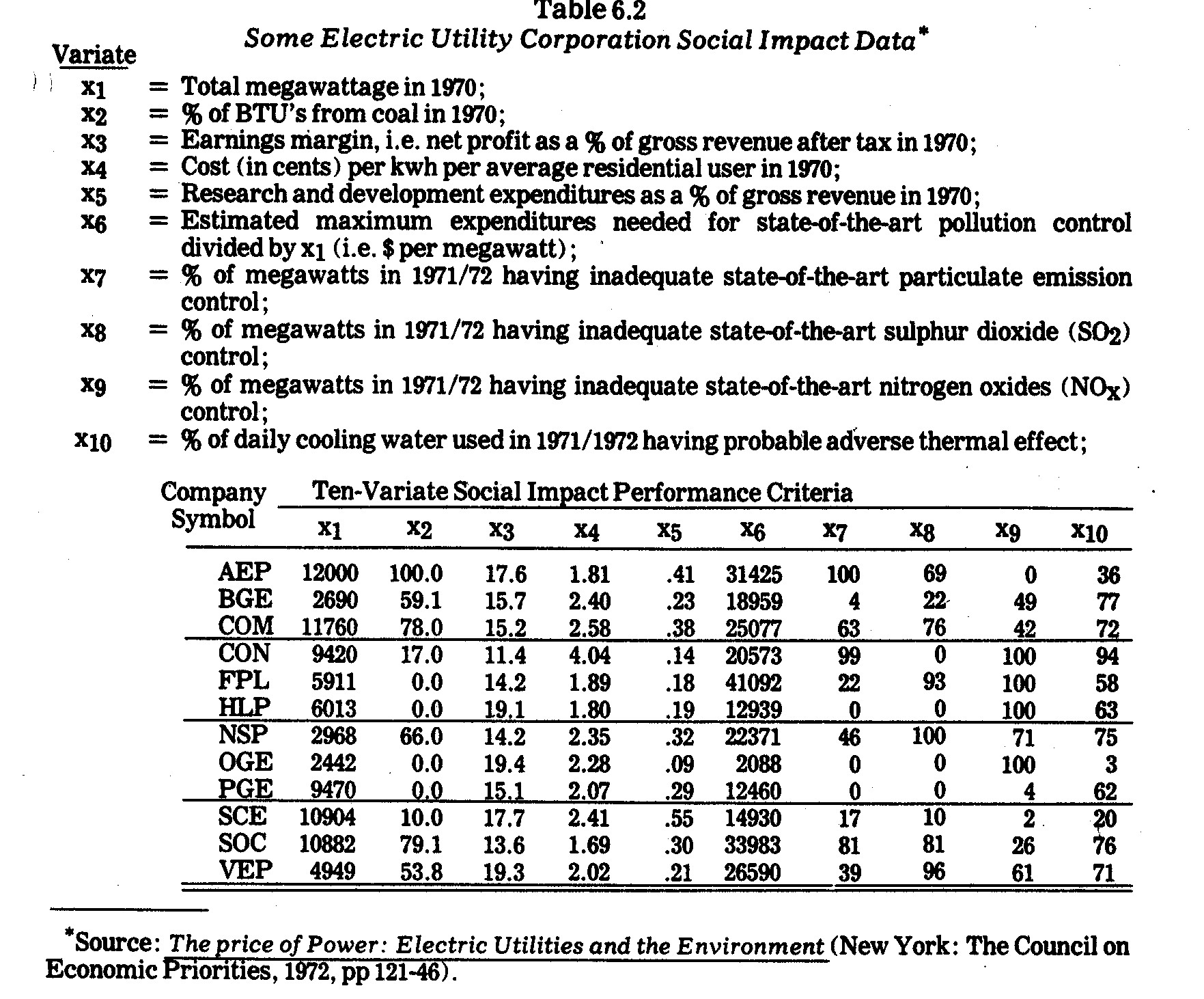
The focal point for many of the illustrations
which follow will be the Table 6.2 data on variates x1,...x10.
It might be noted that except for x1 (megawattage), the other variates x2,...x10
are not necessarily directly associated with size of the companies
involved. For example, whereas pollutant volumes would normally be
expected to increase with the size of an electric power company, percentage data
such as that given for x7,...x10 pollution
variates need not behave in such a manner.
The reader is cautioned about some of the
conclusions which are either explicitly drawn or implicitly inferred in the
illustrations which follow. These conclusions follow only from the data as
tabulated in the Council on Economic Priorities Study. The write-up
for the CEP study contains many footnotes and other explanations on the nature
and limitations of this data. Most of these explanations are not repeated
here but should be carefully heeded before accepting my analysis of the
published data as fact.
In some of the graphical displays it is difficult
to handle more than a few variates at a time. Therefore, from among the
M=10 variates in Table 6.2, a select of subset four social impact criteria was
extracted and is comprised of:
(The Four-Variate Subset)
| x3= |
Earnings margin; |
| x4= |
Cost per kwh; |
| x5= |
R&D proportion; |
| x6= |
State-of-the-art pollution control inadequacy. |
The above four variates cut across various
interest groups, including shareholders, consumers, local communities, and the
public-in-general (who might be especially interested in the R&D
commitment.).
9 Charles
Komanoff, Holly Miller, and Sandy Noyes, The Price of Power: Electric
Utilities and the Environment, Edited by Joanna Underwood, (New York: The
Council on Economic Priorities, 1972).
6.6--Graphic and Other Display Techniques
6.6.1--Purposes. Numerical data are
convenient to view in graphical form whenever possible. For instance,
continuous variates are often displayed in Cartesian scatter plots along one,
two, and occasionally even three dimensions. Discrete data are often
represented in histograms, pie charts, etc. Such display techniques are
familiar and need not be elaborated upon here other than to mention that they
might be effectively employed in corporate social accounting. For example,
wages might be displayed in relation to age, sex, race, plant location,
etc. Pollutant outputs might be plotted in relation to time, weather
conditions, plant locations, etc. Product performance and plant safety
might similarly be displayed in various ways. To date, however, graphic
displays are sparingly employed in corporate social audit reports.
Conversely, in the public sector economic and social indicators are commonly
displayed in graphic form.
Some of the more common purposes of graphical
displays are mentioned below:
-
(COMMUNICATION). Frequently the major
intent is to communicate to other persons as concisely and efficiently as
possible. Graphical displays are advantageous first of all because
they are more likely to capture attention than are long columns of numbers
or paragraphs of text. Secondly, graphical displays are frequently
among the most parsimonious means of communicating data.
-
(DISCOVERY OF DISTRIBUTION PROPERTIES).
Sometimes the analyst constructs a graphical display of a single variate in
order to discover its distributional properties, e.g., dispersion and
skewness. Following a mathematical analysis, outcomes or residuals are
often plotted in order to identify violations of assumptions in the
analysis. For instance, regression residuals are frequently plotted in
an effort to investigate conformance with normality, homoscedasticity, and
independence assumptions.
-
(DETECTION OF ABERRANT PHENOMENA).
Often data are plotted in order to disclose phenomena deviating from
norms. Graphic displays are often a quick and simple means of
detecting awry or extreme reactions.
-
(DETECTION OF LEVEL DIFFERENCES, SHAPES, AND
CLUSTERS). Graphical displays often disclose differences in levels of
observations. However, whereas level differences may often be
discovered by merely scanning the data, hidden patterns, shapes, or clusters
of phenomena may be disclosed (in graphical displays) which are almost
impossible to discern by scanning the data itself.
-
(TRANSFORMATION AND CONCATENATION).
Graphics may assist the analyst in determining what, if any, transformations
of the data (e.g., translation of axes, rotation, and scaling
transformations) provide more useful results. Often these become
linked in a sequence and, through concatenation in interactive computer
graphics, can be combined in one procedure.
-
(INVESTIGATION OF VARIATE AND ENTITY
RELATIONSHIPS). Another purpose of graphical displays may be to
analyze the relationship between two or more variates. For instance,
scatter plots along two dimensions are frequently employed to study linear
or nonlinear relations of two continuous variates. Smooth functions
may be fitted amongst data points. If one of the variates is time, the
purpose may be to identify trends, seasonal patterns, structural shifts, and
drift of a variate of interest over time.
Patterns or clusters may also be detected among
entities. For instance, companies (or divisions within companies) might be
first plotted according to pollutant discharges and then be partitioned into
subsets according to visual scannings of plotted points.
An advantage of visual display is the tremendous
ability and flexibility of humans for detecting spatially and temporally
distributed features in data. Mathematical models, though often an aid in
discovering relationships, have much less flexibility and adaptive innovation
ability.
6.6.2--Limitations. Graphic displays
are physical representations of properties. One limitation is that
qualitative properties are usually cumbersome to display relative to
quantitative properties. Quantitative properties, however, are also
difficult to display in more than two dimensions, even though the analyst is
frequently interested in detecting patterns in multivariate space.
Thirdly, in most graphical displays there is usually an upper bound on the
number of entities that can be effectively plotted and compared. Fourthly,
it is a fallacy to assume that graphic displays are a substitute for
mathematical analysis. Often the detection or communication of phenomena
depends upon making appropriate mathematical transformations of data to be
plotted. Developments in computer graphics have greatly facilitated the
combining of mathematics and graphics.
Various approaches have been proposed for
graphical display to overcome one or more of the above limitations, although
usually trade-offs are encountered. Several of these approaches are
illustrated in the following discussion. In many of these approaches an
added difficulty arises in that how the variates (properties) are assigned to
graphic pattern components either unintentionally or purposefully biases the
outcomes. Also, too many variates may obscure existent patterns in subsets
of the variates.
6.6.3--Profile Line Plots and Shape
Correlations. Although quantitative variates are difficult to plot in
more than two dimensions, various techniques may be employed. One such
technique is profile analysis in which entities are usually compared on the
basis of their "profiles" on two or more variates under study.
Profile analysis is employed extensively in educational and psychological
testing, i.e., persons are compared on the basis of graphical profiles of test
scores. If variates are not measured in the same scales, they are
typically standardized to avoid scaling differences.
For illustrative purposes, four variates (x3,
x4, x5, and x6) were selected from the Table 6.2 data presented previously.
Although the raw data could be plotted in profile charts, I elected to
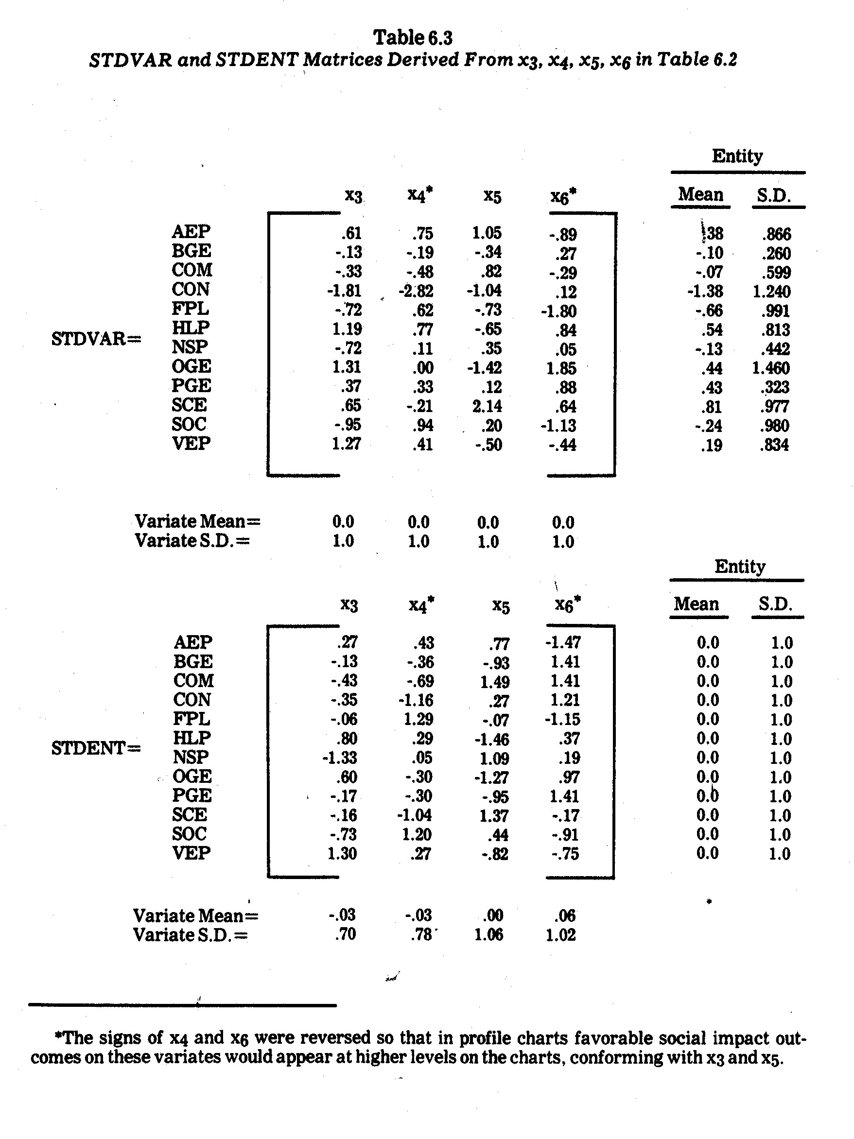
standardize (normalize) the variates using the customary transformation
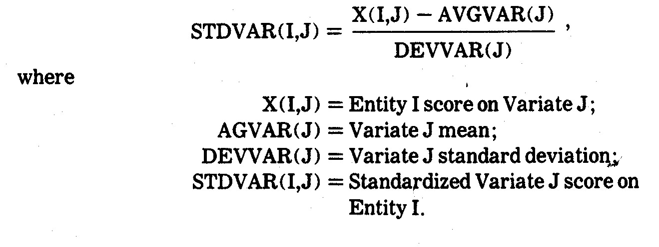
The resultant standardized variate outcomes are
shown in the STDVAR matrix in Table 6.3. The electric utility company
profiles derived from this data are shown in Exhibit 6.1.
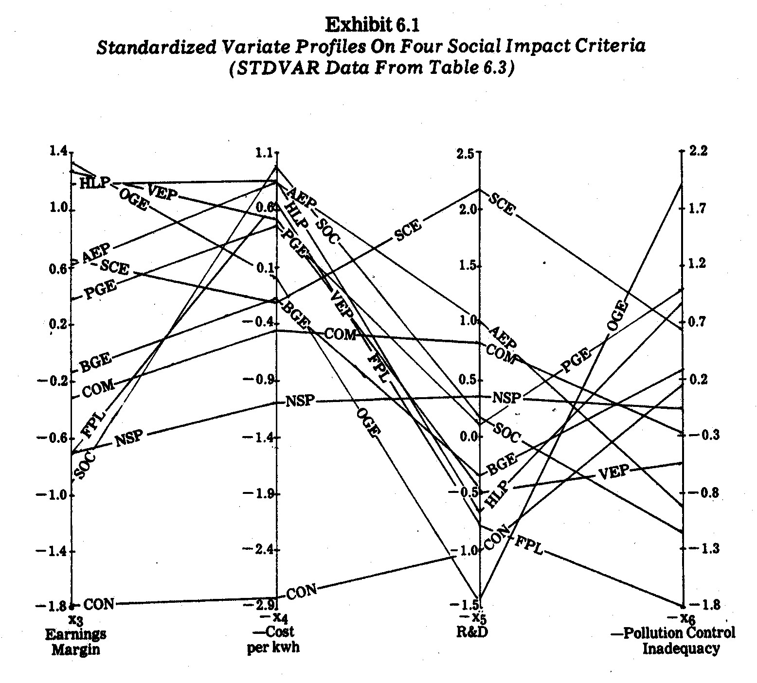
It is immediately evident that no single company
is consistently "best" or "worst" in terms of all four of
these criteria. For instances, Oklahoma Gas and electric (OGE) had the
highest earnings margin (19.4%) and the lowest allocation to research and
development (9% of revenues). Similarly, The Southern Company (SOC)
has a relatively poor performance on three criteria but generates the cheapest
power (1.69¢ per kwh) for average residential users.
On two criteria (earnings margin and price per kwh) Consolidated Edison Company
of N.Y. (CON) falls way below all the other companies in performance.
A careful inspection of Exhibit 6.1 reveals a
number of profile similarities. The Southern Company (SOC) and Florida
Power and Light (FPL) have rather close profiles except for the x5
(R&D) criterion. Houston Lighting and Power (HLP), Oklahoma Gas and
Electric (OGE), and Virginia Electric and Power (VEP) have similar profiles,
especially in terms of the first three criteria. Commonwealth Edison (COM)
and Northern States Power (NSP) have somewhat close profiles on all three
criteria. Pacific Gas and Electric (PGE) and Southern California (SCE) are
also similar except for the x5 criterion (R&D allocation).
These profile similarities seem to suggest
certain geographic "types" since the above-mentioned likenesses are
mostly between companies operating in somewhat contiguous regions. This is
interesting since some of the paired companies along these criteria have major
differences as well, e.g., whereas SOC is a large holding company across various
southern states and in 1970 generated electric power with 79.1% coal, 20.6% gas,
and 0.3% oil, FPL is a much smaller southern company using 56% oil and 44% gas.10
When examining profiles, analysts are sometimes
interested in comparing profile shapes (configurations) irrespective of
differences in profile levels and/or scatter. A transformation which
facilitates such comparisons is the profile scatter transformation
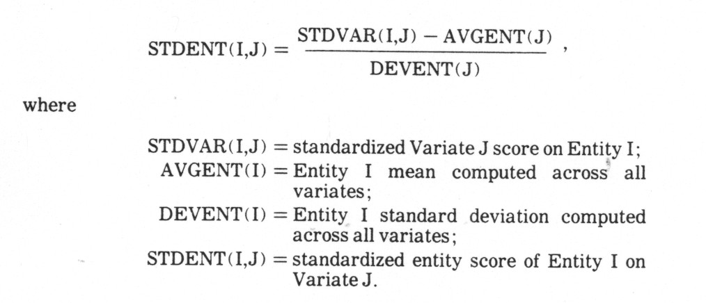
This transformation eliminates both profile level
(elevation) and profile scatter (standard deviation) differences. The
effect of profile elevation removal, in particular, is to bring profiles with
similar configurations (at different levels) closer together.11
The profile scatter transformation yields what are called "pure shape"
proviles.12 Profile charts derived after such a
transformation of the data conform to the profile shape correlation coefficients
computed from the formula

Type your question here and then click Search
This correlation coefficient (sometimes call a
Q-technique correlation) is used when the analyst is interested in comparing
profile shapes aside from elevation and scatter considerations. In other
words, the profile shape correlation coefficients are invariant under profile
elevation and scatter transformations. Other pairwise coefficients (such
as Euclidean distances) are not necessarily invariant under such
transformations, i.e., Euclidean distances reflect differences in profile levels
whereas profile shape correlations measure differences in profile shapes
(configurations).13
10 The Council on
Economic Priorities, The Price of Power: Electric Utilities and the
Environment, Op. Cit., p. 144.
11 From a
mathematical standpoint, the profile elevation transformation (i.e., the
subtraction of entity means) projects the entity scores from N space to a
hyperplane of N-1 dimensions.
12 In mathematical terms,
the profile scatter transformation projects N entity scores to a hypershpere of
N - 2 dimensions of constant radius lying in a hyperplane.
13 The profile
shape correlation coefficients can, however, be shown to be related to Euclidean
distance by the formula
CORENT(I,H) = 1 -
DISENT(I,H))2
_____________________________
2(M - 1)
where DISENT(I,H) is the Euclidean distance
between Entity I and Entity H using STDENT data.
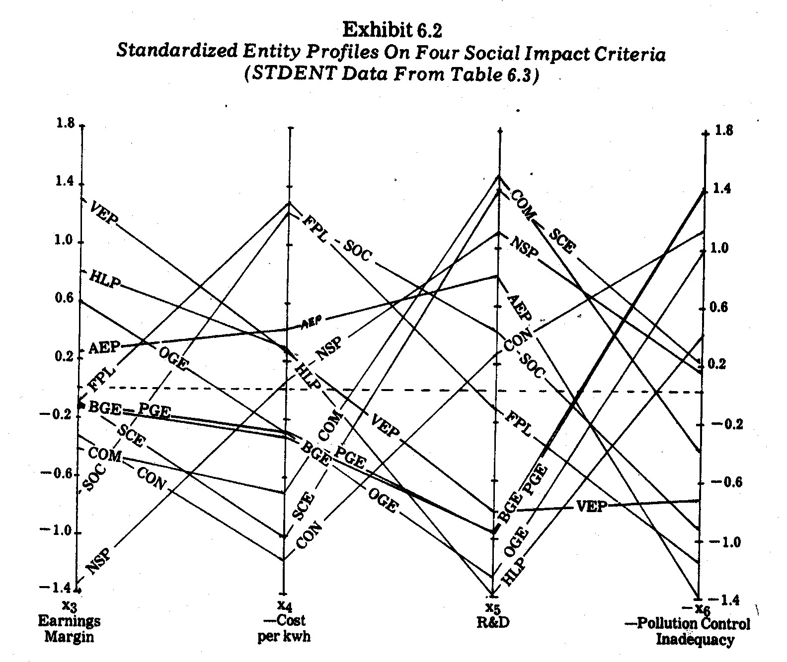
The profile scatter transformation was performed
on the STDVAR data in Table 6.3, yielding the STDENT standardized entity matrix
also shown in Table 6.3. The STDENT profiles are plotted in Exhibit
6.2. One surprising and quite unexpected outcome is the near congruence of
the Pacific Gas and Electric (PGE) and Baltimore Gas and Electric (BGE)
profiles in Exhibit 6.2. This indicates almost identical profile shapes
for these two companies on the four criteria being analyzed, i.e., the two
companies have almost identical profile "shapes" in Exhibit 6.1.
Similarly, the Oklahoma Gas and Electric (OGE) profile is closely related in
shape to both the PGE and BGE profiles. This indicates that these three
companies must also have high profile shape correlations coefficients.
Another surprising likeness in profile shapes, as revealed in Exhibit 6.2.,
arises between Commonwealth Edison (COM) and Southern California Edison (SCE).
In this case, the two companies have similar profile shapes but differ in terms
of profile elevation (in Exhibit 6.1).
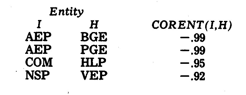
The above visual conclusions from Exhibit 6.2 are
borne out by the profile shape correlation coefficients shown in Table
6.4. The five highest correlations are as follows:
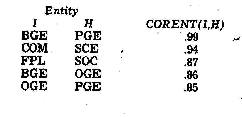
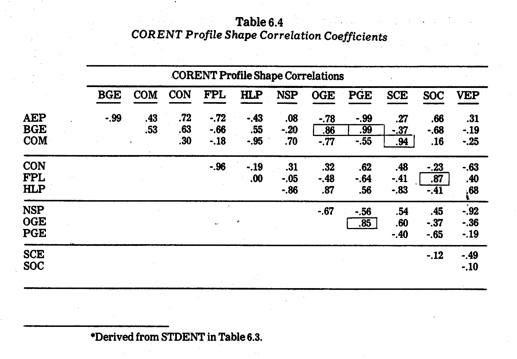
What is a little less obvious in Exhibit 6.2 are
the profile shapes least congruent. In Table 6.4, however, the most
negative profile shape correlation coefficients are revealed as:
These differences are not especially surprising
except for the Northern States Power (NSP) and Virginia Electric Power (VEP)
profiles. These two companies are somewhat similar in size and in fuel
usage.14 However, whereas the NSP profile in Exhibit 6.1
is relatively flat, the VEP profile moves from a high on earnings margin and
cost per kwh to lows on R&D and pollution control inadequacy.
14 In 1970,
the fuel use for NSP was 66% coal, 33% gas, and 1% oil. For VEP the
percentages were 53.8% coal, 46% oil, and 0.2% gas.
6.6.4--Principal Component (Factor Score)
Profiles. Profile analysis becomes clumsy when more than five or six
variates (criteria) are under study, e.g., imagine trying to compare profile
patterns over twenty or thirty social criteria. Often, however,
multicollinearities exist such that one, two, or several principal components or
factors account for much or most of the variation in an entire system of
variates.
One approach is to transform the original
variates into factors and then plot entity factor scores. For one or two
principal factors, entities can be plotted in scatter plots. For more than
two factors, entity profile configurations can be examined using underlying
factors in lieu of original variates.
Suppose there are M variates under study.
There are two major reasons why factor scores may be more of interest than
original data:
(1) Whereas the M variates under study may be
systematically intercorrelated with one another, the factors (principal
components) are linearly independent (orthogonal). This is helpful in
data analysis techniques which are linearly independent (orthogonal).
This is helpful in data analysis techniques which assume linear independence.
(2) The factors (principal components) are extracted in such a manner that
they successively account for smaller portions of the total variation among
the M original variates. If the first few factors account for a large
share of this variation, and if they can be meaningfully interpreted, it may
be possible to describe the system more parsimoniously (i.e., in fewer than M
variates).
The major difficulty in principal component or
factor analysis often lies in interpreting the importance and meaning of the
factors extracted from the original variates. The relative importance of
successive factors can be estimated by comparing their latent roots (eigenvalues).
Finding descriptive interpretations is more difficult. The usual approach
is to examine the factor loadings (eigenvectors), which are correlations between
factors and original variates. Frequently, subsets of the original
variates having highest correlations with a given factor have something in
common which is suggestive of what the factor depicts.15
15 This
approach was illustrated in the Chapter 4 principal component analysis of air
pollution and human mortality data. An excellent elementary example is
also provided in W. W. Cooley and P. R. Lohnes, Multivariate Data Analysis
(New York: John Wiley & Sons, Inc., Second Edition, 1971, pp. 133-36).
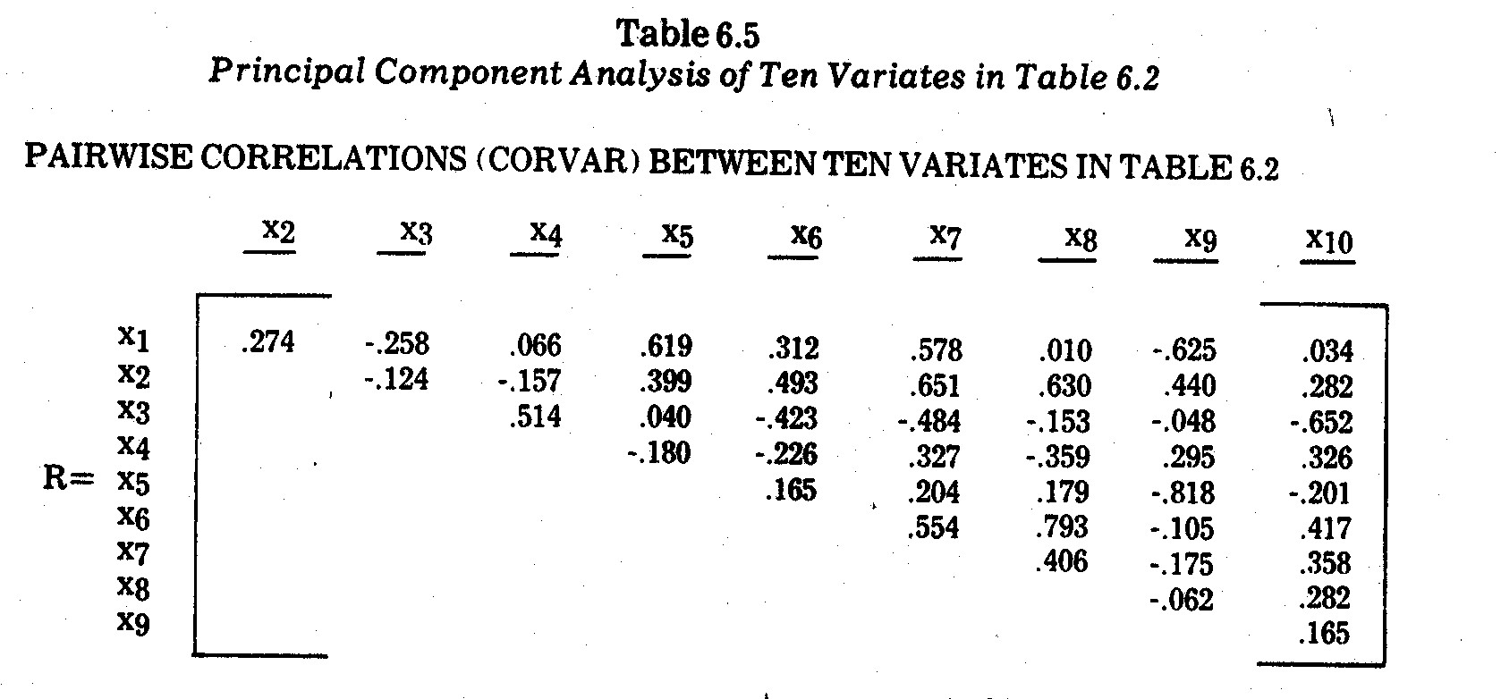
For illustrative purposes, the pairwise
correlations between variates x1,...,x10 given in Table
6.2 are given in the CORVAR matrix in Table 6.5. An underlying factor
structure is not easily determinable from merely scanning this correlation
matrix. A
I. PAIRWISE CORRELATIONS (CORVAIR)
BETWEEN TEN VARIATES IN TABLE 6.2
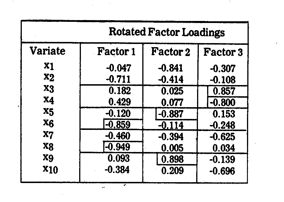
II. FACTOR LOADINGS
III. FACTOR INTERPRETATIONS
(1) Factor 1 (Air Pollution Control
Inadequacy): This factor loads highly on overall pollution inadequacy (x6)
and sulphur dioxide control inadequacy (x8), both of which reflect
air pollution under-investment in state-of-the-art controls available.
This factor also loads relatively high on coal usage (x2), suggesting
that heavy coal burning companies have a more serious under-investment in such
controls, although there is considerable dispute over what constitutes
"state-of-the-art" control, e.g., the wet scrubber dispute is
discussed later on.
(2) Factor 1 (Technology): This appears
to be largely an R&D (x5) and nitrogen oxides control
inadequacy (x9) factor, the two variates being highly correlated at
-.818. Size of company in terms of megawattage (x1) also
loads highly on Factor 2, partly reflecting the fact that there is a tendency
for larger companies to have a higher R&D proportion and lower nitrogen
oxides control inadequacy.
(3) Factor 3 (Financial): This appears
to be a combination of the company's earnings margin (x3) and
average customer price per kwh (x4), the two being negatively
correlated at -.5145.
(4) Factor 4 thru 10 (Junk): These
factors have latent roots less than one, and hence, are not viewed as relevant
underlying factors.
IV. LATENT ROOTS (EIGENVALUES)
| Factor |
Latent Root |
Variance
Accounted For |
| |
|
Percentage |
Cumulative |
| 1 |
2,7466 |
27.466% |
27.466% |
| 2 |
2,6882 |
26.882% |
54.348% |
| 3 |
2,4751 |
24.751% |
79.099% |
| 4-10 |
2,0901 |
20.901% |
100.000% |
principal component analysis on the variates x1,...,x10
in Table 6.2 yielded the outcomes in Table 6.5. Three factors emerged with
latent roots exceeding one. These three factors account for 79.1% of the
variance in the ten-variate system. Interpretations of these factors are
not at all obvious or concise. Based upon the rotated factor loadings
shown in Table 6.5, the best interpretations I could come up with are also given
in Table 6.5.
The illustration points out one of the potential
frustrations with principal component or factor analysis in general, i.e., a
frequently encountered situation arises in which there is no concise and
all-embracing concept for two or more rather heterogeneous variates closely
correlated with a factor. This is particularly evident in Factor 2 in
Table 6.5, which loads highly on research and development (x5),
nitrogen oxide control inadequacy (x9), and megawattage (x1).
It is also evident in Factor 3, which loads highly on earnings margin (x3)
and cost (price) per kwh to an average residential electricity consumer (x4).
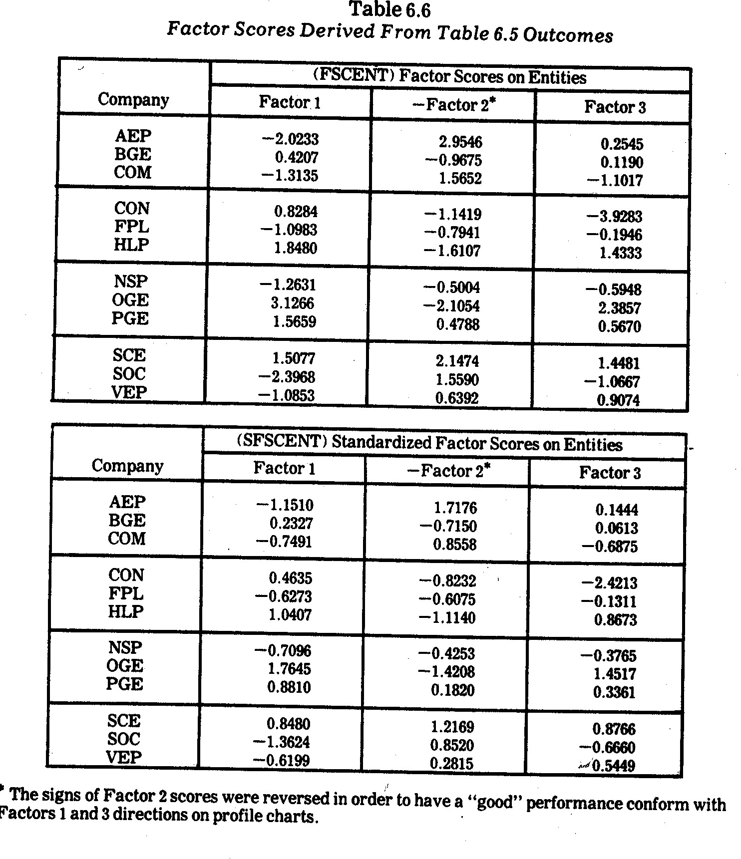
The outcomes in Table 6.5 were utilized in
transforming the M=10 variates (in Table 6.2) into the major factor scores (on
each entity) sown in Table 6.6. The company (entity) profiles derived from
the standardized factor scores (SFSCENT) are shown in Exhibit 6.3. No
company consistently performs highest on all criteria, although SCE performs
relatively well on all three major underlying factors, brief interpretations for
which were given in Table 6.5. The inconsistent performance of CON is
manifested in its somewhat reasonable performance on Factor 1 (pollution
control) relative to falling way below other companies on Factor 3 (financial
performance) due to a combination of having both the lowest earnings margin and
the highest kwh rates. The inconsistent performance of AEP is also evident
in its poor showing on Factor 1 (pollution control) relative to the highest
showing on Factor 2 (technology) due to a combination of having a relatively
high R&D commitment (x5) and a low nitrogen oxides
state-of-the-art underinvestment (x9). As indicated previously,
however, the AEP performance on x9 is misleading since it is the lack
of technology for "state-of-the-art" pollution control rather than
investment in pollution controls which gives the coal-fired AEP such a good
score on x9.
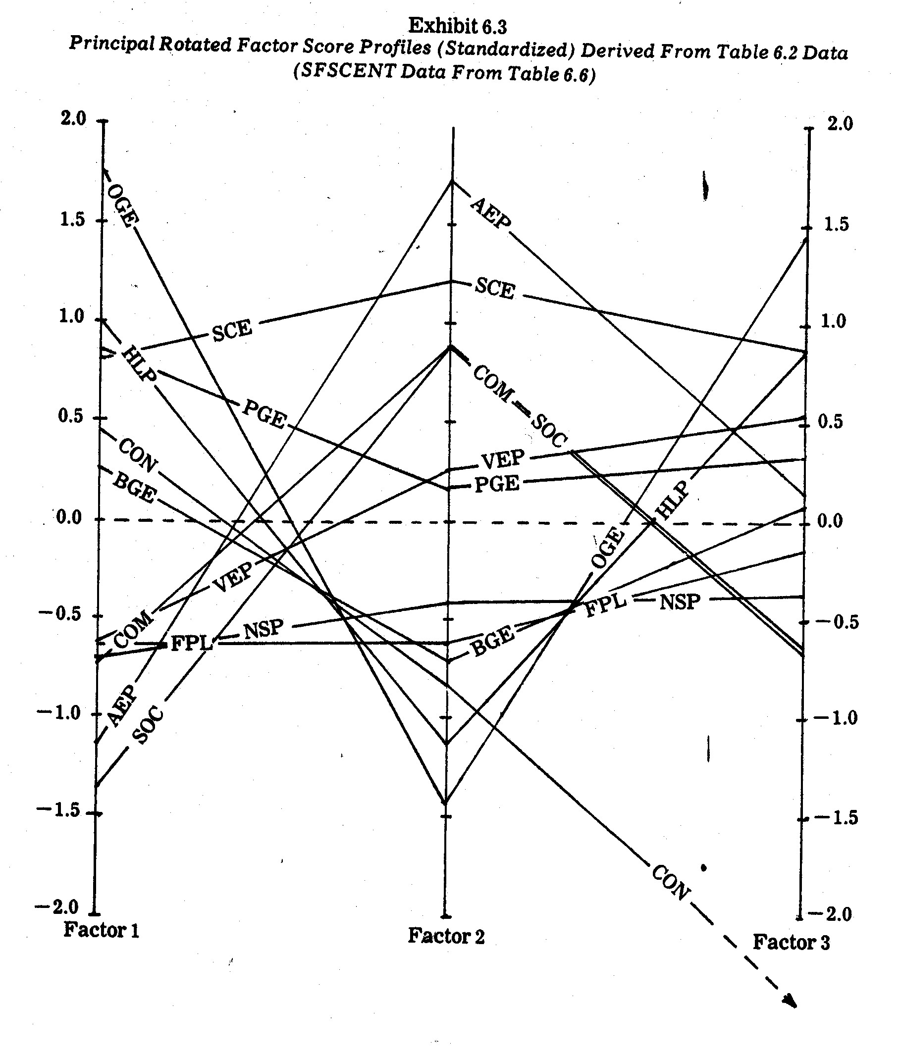
Similarity in both level and shape on the three
principal underlying factor profiles in Exhibit 6.3 are also evident. For
example, the large coal burning companies (AEP, COM, and SOC) have very similar
profiles, with AEP pulling ahead on Factor 2 due to a higher R&D
commitment. In contrast, the smaller natural gas-fired OGE and HLP
companies have almost congruent profiles with shapes nearly opposite those of
the large coal-fired companies. The larger SCE, however, does not succumb
to the OGE and HLP drop along Factor 2 because of the exceptional performance of
SCE on both R&D (x5) and nitrogen oxides (x9)
criteria.
One of the most important outcomes in the factor
score profiles in Exhibit 6.3 arises in the amazing similarity between the
Florida Power and Light (FPL) and Northern States Power (NSP) profiles.
In contrast, the M=10 variate raw scores for these companies (see Table 6.2) are
much more divergent.16 This phenomenon provides an
important illustration of how principal components or other types of factor
analyses can be used to reduce a large number of variates into a more
parsimonious subset of underlying principal factors. At the same time it
also illustrates "overkill" in the sense that the outcome may be
too parsimonious. For example, the primary determinants of Factor 3
appear to be quite different social impact criteria which, at least in this
data, are negatively correlated. Company scores on Factor 3 are caught
between opposing forces. For example, the FPL "poor" showing on
earnings margin (x3) pulls against the FPL "good" score on
electricity pricing (x4). Similar negative correlations in
performance criteria are present in other factors. Hence, this is the case
where, because of opposing interests in given factors, less parsimony in terms
of keeping opposing criteria separated is probably more meaningful.
16 Also note
the divergent FPL and NSP profiles in Exhibit 6.1.
6.6.5--Fourier Series Profiles. In
the preceding section, a principal component analysis was reported in which M=10
variates were parsimoniously reduced to M'=3 factors (principal
components). The resultant factor scores were plotted in the Exhibit
6.3. Suppose, however, that such an analysis yielded a substantially
larger number of underlying factors, e.g., suppose M=50 variates produced M'=15
factors of interest. Profile charts are difficult to construct and
evaluate for more than a few factors.
An alternate approach which is especially
interesting when there are more than a handful of underlying major factors is to
use a Fourier series method originally proposed by Andrews.17
The procedure for plotting multivariate observations on each entity is to
compute the following Fourier series transform on each entity (e.g., each
company):
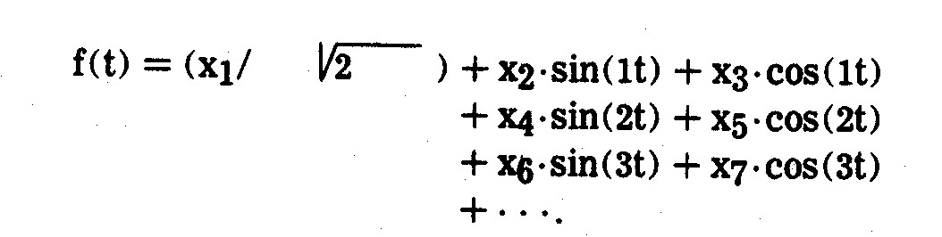
The f(t) function is then plotted (best results
are obtained from a computer plotter) for values of t over the range ±3.1416, such that each entity receives a
plotted curve over this range of t. Profiles of entities may then be
compared both as to level and to configuration. The number of variates is
not a limiting constraint, i.e., the f(t) function is plotted against t rather
than the xJ variates. When the xJ variates are
linearly independent and certain other assumptions are met, the f(t) outcomes
have a number of interesting properties and are conducive to statistical
inference testing of differences between entity profiles.
Proceeding
by way of illustration, consider the factor scores shown previously in Table
6.6. These outcomes were transformed into Fourier series curves plotted in
Exhibit 6.4. Most plotted f(t) profiles yield conclusions similar to those
derived previously from the profiles in Exhibit 6.3. For example, in
Exhibit 6.4 the FPL(E) and NSP(G) curves are nearly congruent, indicating that
these two companies have almost identical scores on the three major underlying
factors. The similarity among the three largest coal-fired companies (AEP(A),
COM(C), and SOC(K)) are also evident in their bell-shaped curves which differ
markedly from the curves of the other companies. The natural gas burning
companies HLP(F) and OGE(H) also have similar profiles. The widely
differing performances of CON and SCE are also evident.
When
there are only a few factors (e.g., the three factors in Exhibit 6.3) there
seems to be little advantage in resorting to the more complex Fourier series
profiles such as those in Exhibit 6.4. The Fourier series approach becomes
more interesting when the number of factors becomes too unwieldy for a profile
analysis on all factors simultaneously. However, both approaches (e.g.,
those in Exhibits 6.3 and 6.4) are cumbersome when there are very many entities,
e.g., the N=12 profiles plotted in the preceding profile exhibits approach the
limit of human ability to visually compare profiles.

17 D. F.
Andrews, "Plots of High Dimensional Data," Biometrics, Vol. 28,
March 1973, pp. 125-36.
6.6.6--Geometric Patterns and Plotted
Caricatures. Instead of plotting multivariate data as scatter plots or
profile line plots, it is sometimes better to consider other geometric patterns
(e.g., triangles, rectangles, etc.) or caricatures (e.g., facial
sketches). It may be particularly advantageous to do so when:
(1) The number of entities (N) is such that
profile lines overlap and crisscross so much that entity comparisons are
difficult, e.g., previous profile plots of N=12 electric utility companies
were difficult to evaluate because of numerous intersecting line segments.
(2) There are discrete qualitative variates under study which can be depicted
as varying geometric shapes or caricature components.
There is a limit to how many entities (N) can be
depicted or how many variates (M) can be incorporated as features in geometric
patterns or caricatures. In recent years, however, a number of interesting
innovations in these areas have arisen, some of which will be illustrated here.
For example, Edgar Anderson proposed the drawing
of geometric patterns which he termed "glyphs."18
These were intended primarily for the graphical display of multiattribute
discrete variates in biology. A glyph has a base (or core) with rays
pointed upward, where each ray depicts a different attribute. For example,
an attribute having three categories is depicted by Anderson as a ray having
three lengths, i.e., zero, medium, and long.
A slightly modified glyph approach is illustrated
in Exhibit 6.5. In this case the standardized variates on x3, x4,
x5, and x6 social impact criteria in Table 6.3 are
depicted as separate rays (in clockwise order). Each glyph corresponds to
a different electric utility company. The ray lengths are marked into unit
gradations where:
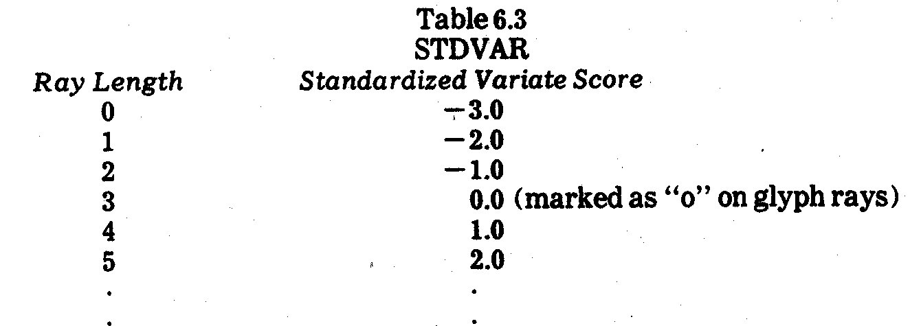
The origin on a standardized variate (which is
also the mean of a standardized variate) is marked with a "o" on those
rays for which companies scored at or above the mean on the criterion in
question.
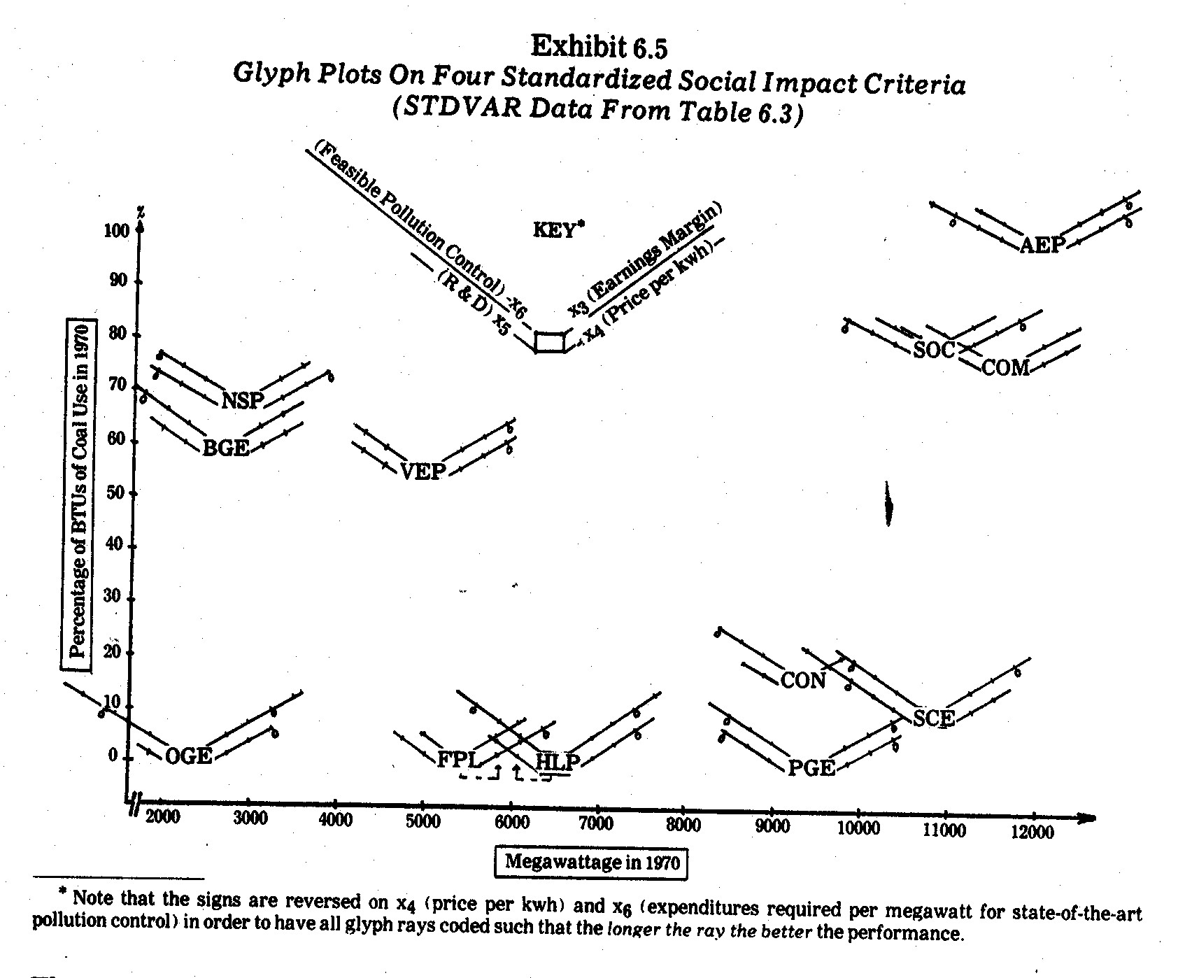
In Exhibit 6.5 each glyph is plotted in a
two-dimensional Euclidean space, where the horizontal axis corresponds to x1
(megawattage) and the verticle axis corresponds to x2 (coal usage)
raw data scores from Table 6.2. Note that the largest coal burning
companies (AEP, COM, and SOC) are isolated by themselves in x1 and x2
space. Smaller companies which also rely heavily on coal (NSP, BGE, and
VEP) also cluster by themselves. Companies which use little or no coal are
also clustered on the x1 axis as large (SCE, PGE, and CON), medium (HLP
and FPL) and small (OGE).
The net result is that in Exhibit 6.5
multivariate data in six dimensions are plotted in two-dimensional space.
The company glyphs resemble frontal views of wounded biplanes returning from
battle. Performances on the x3, x4, x5, and
x6 standardized criteria
appear as wings (rays) of varying lengths. If the origin, "o,"
is shown on the wing (ray), the company performed at or above the mean on the
criterion in question. The "o" origins resemble engines beneath
a wing. In this context, a company has an "engine" on a wing if
it performed at or above the mean performance on that criterion.
In this sense, the "best" performing
companies in Exhibit 6.5 are those with the longest wings. The only
company performing above the standardized mean (zero) on all four social impact
criteria (and therefore having all four "engines" intact under its
glyph wings) is Pacific Gas and Electric (PGE). Both HLP and OGE are
natural gas burning companies which perform at or near the best on three
criteria (x3, x4, and x6) but have little or no
wing (ray) length on the x5 (R&D) criterion. Similarly, SCE
performs quite well on three criteria but falls slightly below the mean on the x4 (kwh price) criterion. AEP and NSP are also "three-engine"
glyph biplanes, where AEP falls short on x6 (pollution control
inadequacy) and NSP falls short on x3 (earnings margin).
In contrast, CON barely flies along on its single
x6 (pollution control inadequacy) engine whereas FPL limps on its x4
(price per kwh) performer. Other single-engine glyphs (BGE and COM) have
better balance in terms of wing (ray) length on all four criteria in Exhibit
6.5.
Among all the graphic display approaches
illustrated thus far, I find the glyph approach quite appealing.
Anderson's glyph rays are plotted according to discrete ordinal scales, although
nominal or continuous (as illustrated in Exhibit 6.5) variates may be plotted as
glyph rays. Glyphs may also be used as geometric pattern representations
without having to be plotted in Euclidean space. Anderson recommends no
more than seven rays and that rays do no extend in all directions.
He also recommends having no more than three discrete levels for ray length (a
recommendation which was not followed in Exhibit 6.5). Continuous variates
may also be transformed into these three discrete ordinal categories.
Multiple rays may be used for more than three categories or complexes of related
variates. Anderson writes:
In attempting to work out complexes of related
qualities, the analysis is facilitated if the ray lengths are coded in such a
way that all the extreme values characteristic of one complex are assigned
long rays and those characteristic of the other are assigned no rays.
For example, in studying hybridization between two subspecies of Campsis, one
of the subspecies had a short tube, a wide limb, and much red in the flower;
the other had a long tube, a small limb, and little red. Redness and
limb width were coded with long rays for much red and for wide limbs, tube
length was coded in reverse with a long ray for short tubes. This meant
that those hybrids closely resembling the other parent as (sic.) a rayless
dot.19
For purposes of graphic plotting, the symbols
drawn may be triangles, line segments, polygons, or most any caricature
imaginable. One of the most unique caricature plotting ideas is described
by Tversky and Krantz.20 They depict alternate sketches
of face shape (long versus wide), eyes (empty versus
filled-in), and mouth (straight versus curved) to represent three binary
variates in two-dimensional plots. The facial sketches were then used in a
visual perception test of interdimensional additivity, i.e., that overall
dissimilarity between faces could be decomposed into additive components
represented by varying facial features.
A more extensive and general facial plotting
program was apparently developed independently by Chernoff,21
although both Tversky-Krantz and Chernoff utilize elliptical components.
Each variate (initially the computer program developed by Chernoff can handle up
to 18 variates, but the program can be modified to accommodate more variates) is
represented as a feature (eye shape, eye size, mouth shape, mouth size, etc.) in
a computer-sketched face. Differing values of the variate are
distinguished by different sizes and/or shapes of the feature in question.
Each entity is depicted by a particular face whose features are determined by
observed values of variates on that entity. An advantage of facial
caricatures over glyph plots is that numerous features can be depicted in faces
whereas Anderson found that glyphs with more than seven rays were too
cumbersome.
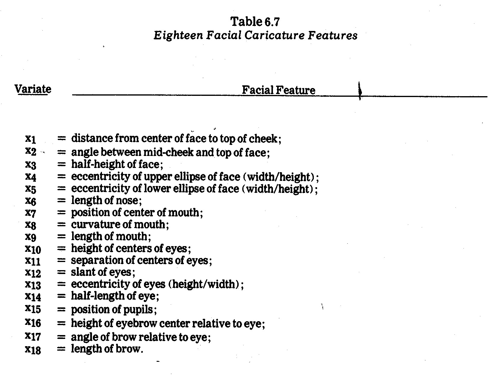
The facial features in Chernoff's original
program are listed in Table 6.7. If there are fewer than M=18 variates
under study, a given variate may (i) be assigned to more than one feature or
(ii) certain features may remain fixed.
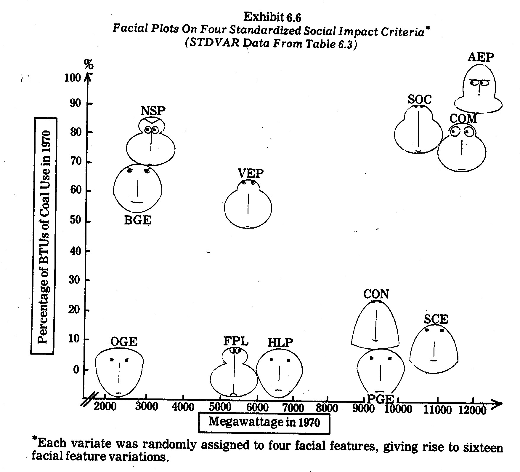
For instance, the N=12 entities (electric utility
companies) measured on M=4 social impact criteria in Table 6.3 are plotted as
faces in Exhibit 6.6. In this case the M=4 variates were randomly assigned
to four different facial features, giving rise to 16 features which vary among
the N=12 faces plotted in Exhibit 6.6. The faces have been arranged in
two-dimensional Euclidean space on x1 (megawattage) and x2
(coal usage) from Table 6.2, i.e., the exhibit depicts two Cartesian variates
and sixteen facial variations determined by x3 (earnings margin), x4
(kwh pricing), x5 (R&D), and x6 (pollution control
inadequacy). Recall that the latter four criteria were also displayed in
Exhibits 6.1 and 6.2 in profile charts and Exhibit 6.5 as glyph rays.
After plotting the faces, I had a number of
students, businessmen (e.g., those who attended my N.A.A. courses on accounting
for corporate social responsibility22), and other friends try
to match up the faces. For this purpose the faces were not plotted in
Euclidean space on x1 and x2 as they are in Exhibit 6.6
nor was there any indication as to what the faces depicted. Interestingly,
rather consistent partitionings of these N=12 faces into G=5 clusters (groups)
emerged from those subjective evaluations.
The most consistent clustering
were as follows:
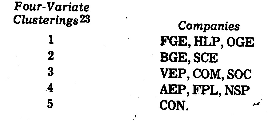
Variations in the above clusterings tended to
arise mainly in differing partitionings among the Cluster 1 and 2 companies, all
of which tend to be the "good guys" in terms of Table 6.3 data
relative to the companies in Clusters 3, 4, and 5.24 In
any case, the subjective clusterings differed greatly in terms of x1
size and x2 coal usage variates (see Exhibit 6.6). For example,
BGE is a small and relatively heavy coal user whereas SCE is a much larger power
company with only light usage of coal. Similarly, AEP, NSP, and FPL vary widely in terms of
size and/or coal usage. It might also be noted that I tended to get fairly
consistent outcomes when human subjects clustered faces obtained under two other
random assignments of particular facial features to the M=4 social impact
criteria in Table 6.3.
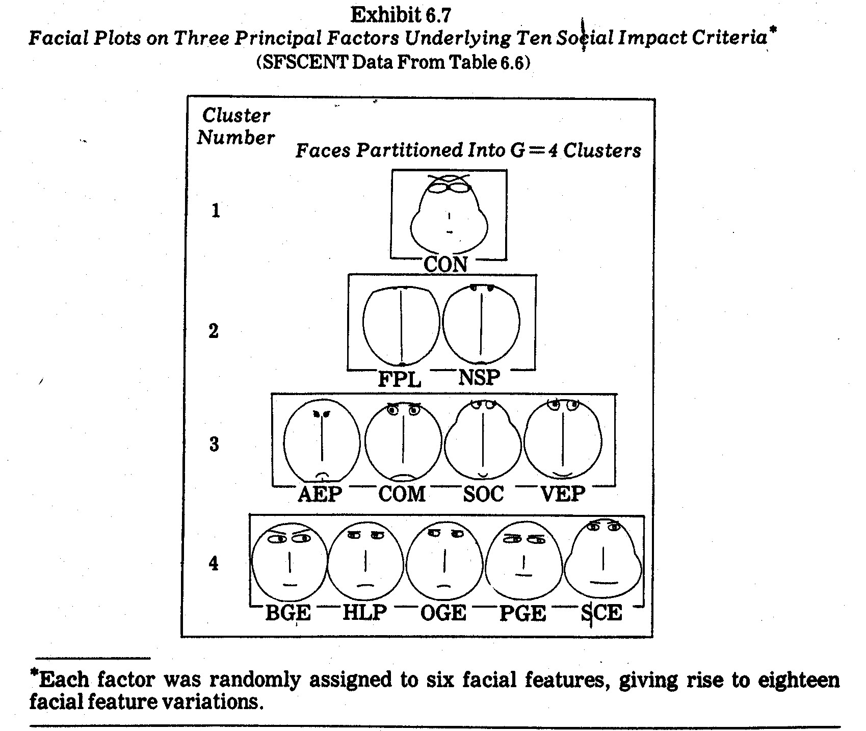
In a second effort, I used the standardized (SFSCENT)
factor scores in Table 6.6 (which in turn were derived from the M=10 social
impact criteria in Table 6.2) to obtain the electric utility company faces shown
in Exhibit 6.7. The most consistent subjective clusterings (among the
human subjects I persuaded to match up the faces) correspond to companies
allocated to G=4 clusters (groups) as follows:
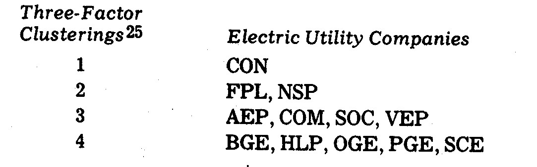
Faces are grouped in Exhibit 6.7 to reflect these
clusters. Variations arose mainly when a few subjects matched CON, SOC,
and SCE, apparently on the basis of head shape but ignoring major differences in
length of nose, length of mouth, height of centers of eyes, separation of
centers of eyes, half-length of eyes, position of pupils, eccentricities of
eyes, and eyebrow features.26 The fact that some persons
matched CON, SOC, and SCE faces highlights the need to make several plottings of
faces with different random assignments of variates (in this case factors) to
facial features. The Exhibit 6.7 faces are the result of only one such
random assignment.
The more frequent clusterings of faces into G=4
clusters (groups) shown in Exhibit 6.7 conform fairly well with the Exhibit 6.3
profiles. Both FPL and NSP faces are closely matched in Cluster 2, whereas
CON by itself in Cluster 1 stands apart from the rest of the faces in feature
combinations. The Cluster 3 companies AEP, COM, and SOC have similar
profiles in Exhibit 6.3, whereas the VEP difference in profile shape is not
reflected in the Exhibit 6.7 faces. In order to capture profile shape
comparisons it would be better to first remove entity elevation and scatter (to
arrive at STDENT values in the manner described previously) before plotting the
faces.
Cluster 4 in Exhibit 6.7 contains the least
homogeneous profiles (from Exhibit 6.3). In particular, BGE, HLP, OGE, and
PGE are joined together, whereas both the BGE and PGE profiles differ rather
markedly from the HLP and OGE profiles in Exhibit 6.3. Once again this
demonstrates that, if profile shape (rather than level) is of primary interest,
a profile scatter transformation should be made prior to forming the
faces. Cluster 4 does tend to contain the "clean-guys" with
higher proportions of natural gas-generated electric power. The noteworthy
exception in Exhibit 6.7 cluster 4 is Baltimore Gas and Electric (BGE) which in
1970 utilized 59.1% coal as opposed to 0.1% gas. In terms of size and coal
usage, BGE is much more like NSP and VEP, but its face (and its standardized
principal factor scores) differs markedly from the NSP and VEP faces in Exhibit
6.7.
An apropos question is (among the infinite
patterns or caricatures which might be used)--"Why faces?".
Probably the best argument which might be raised in favor of faces is that all
people with sight are used to seeing faces. At an early age humans learn
to distinguish, on the basis of manifest facial features, hundreds or even
thousands of faces (both real and cartoon). A second argument is that
numerous variates can be depicted by facial features (jaw line, cheeks,
nose, eyes, ears, hair, dimples, wrinkles, etc.) in terms of shape, size, and
orientation. If additional body features (neck, chest, abdomen, etc.) are
added in, thousands of variates can, in theory, be included. Prior to
computer-aided plotting, however, slight variations in continuous variates would
have been difficult to precisely portray.
It is usually possible to compare more entities
in caricature plotting than in profile analysis. Chernoff, for example,
provides two empirical illustrations comprised of 88 and 53 entities (faces)
respectively.27 A visual cluster analysis was attempted
by various persons in both instances, with consistent agreement on clusterings
of Chernoff's many facial caricatures.
There is a limit, however, to how many faces can
be visually compared and clustered by human analysts. I cannot imagine,
for example, comparing N=729 caricatures in the Pickett and White study to be
mentioned later on, i.e., if faces were drawn smaller and condensed for
"texture' comparisons, features in each face would be obscured. Thus,
the facial caricature approach would probably be used for a fewer number of
individual comparisons, although the maximum upper bound of faces that can be
compared depends upon many circumstances.
Another drawback of the facial caricature
approach, it seems to me, is that in a given facial feature only extreme
variations are easily discerned. This can be partly overcome by assigning
a variate to two or more features which, in combination, serve to bring out
lesser variations.
Still another drawback is that some facial
features may have more importance than others in distinguishing faces.
This implies that clustering outcomes may may be biased
when assigning variates to facial features. This can be partly overcome by
repeating the analysis several times under alternative assignments of variates
to features. This approach, of course, increases the time, effort, and
cost of the study in terms of computers, plotters, and persons examining facial
caricatures.
An especially bothersome phenomenon in both
profile and pattern display approaches (including facial caricatures) is that
the addition of too many variates may tend to obscure patterns in smaller
subsets of the variates under study. The solution seems to fall back on
repeated attempts under judicious selections of subsets of variates. In
this regard, statistical analysis and graphic analysis might work
hand-in-hand. For instance, a multiple regression might be performed to
"take out the effects" of certain variates (as in covariance analysis)
prior to plotting regression residuals. Similarly, a principal component
analysis might be performed in order to extract interpretable orthogonal factors
to be used in lieu of intercorrelated variates. This latter approach was
illustrated previously in Exhibit 6.7.
18 Edgar
Anderson, "A Semigraphical Method for the Analysis of Complex
Problems," Technometrics, Vol. 2, August 1960, pp. 387-91.
19 Ibid,
p. 391.
20 Amos
Tversky and David H. Krantz, "Similarity in Schematic Faces: A Test of
Interdimensional Additivity," Perception and Psychophysics, Vol. 5,
1969, pp. 124-28.
21 Herman
Chernoff, "The Use of Faces to Represent Points in n-Dimensional Space
Graphically," Technical Report No. 71, Department of Statistics, Stanford
University, December 27, 1971. Portions of this paper are also published
in the Journal of the American Statistical Association, June 1973, pp.
361-68.
22 These
N.A.A. courses were mentioned in greater detail in Chapter 3.
23 Using Exhibit
6.6 faces, which in turn were derived using STDVAR data from Table 6.3 on x3,
x4, x5, and x6. I hesitated to conduct a
formal analysis of the subjective clusterings for a number of reasons, one of which
is that time constraints under which subjects were asked to compare faces varied
greatly due to circumstances outside of my control. Only 33 persons
submitted completed subjective clusterings according to my instructions, which
allowed them to choose both the number of clusters and the assignment of faces
to clusters. The mode clustering outcome (12 cases) was that shown
above. Variations tended to not differ greatly from this mode.
24 There are
exceptions noted previously, however, such as the low R&D commitments (x5)
of HLP and OGE relative to AEP and COM. The ultimate judgment of
"good versus "bad" entails consideration of other criteria
and operating constraints.
25 The three
factors (components are the Table 6.6 standardized factor scores underlying the
M=10 variates in Table 6.2. I hesitated to conduct a formal analysis of
subjective clustering variations for reasons noted previously.
26 Each of the
three standardized factors (from Table 6.7) was randomly assigned to six facial
features giving rise to eighteen facial feature variations in Exhibit 6.7.
27 The first
of these involved eight variates observed on each of 88 specimens from the
Encene Limestone Formation in northwestern Jamaica. The second involved
twelve variates observed on each of 53 mineral core specimen from a core drilled
in a Colorado mountainside. In both instances the variates were all
quantitative in nature.
6.6.7--Texture Analysis in Large Sample
Graphs. If geometric patterns or caricatures are to be compared for a
large number of entities, comparisons of individual entities may become futile
(unless the intent is to discover one or a few aberrant entities which stand out
from the crowd). In such instances, however, it may be possible to
identify patterns among dense groupings of entities. In information
display terminology this is sometimes called analyzing the "texture"
patterns. For example, Pickett and White28 use
computer-graphic triangles to represent N=729 college students. The
triangles are drawn quite small in order to fit on a single page. Each
triangle depicts five variates in the manner described below:
Each triangle presents five measures. Two
of the measures control the position of the triangle in its unmarked 30x30
raster unit cell. Another measure controls the altitude of the triangle,
another its orientation and another the width of its base.29
Whereas in preceding Exhibits 6.1 thru 6.7,
individual entity (company) profiles could be compared with one another, it is
difficult to imagine such comparisons among the mass of N=729 triangles
(depicting college students) drawn by Pickett and White. Many of their
triangles are so small that their plot is hardly more than small, faint
lines. Instead of individual comparisons, the Pickett and White approach
is normally used to compare predefined groups or classes of entities. For
this reason, entities are arranged in the Pickett and White illustration as
described below:
The data are arranged into three groups,
forming verticle bands of equal width. The left band contains profiles
of dropouts, the middle band profiles of regular graduates, the right band
profiles of honor graduates.30
From these outcomes, Pickett and White concluded
the following:
Again the hope would be that some new hints of
differences among these three groups might be derived by looking at such a
display. One intriguing thing that has been suggested by brief perusals
so far is that honor students may be more similar to dropouts than they are to
regular graduates. It is insights of this rather unexpected sort which,
if they prove to be valid, would make such a regular display technique very
much worth while.31
In graphic displays with densities such as that
illustrated by Pickett and White, the images resemble something analogous to the
texture of interwoven or interwined threads. Human perception of visual
"texture" has been the subject of behavioral study.32
The objective might be to perform either:
(i) Cluster Analysis--to
identify similar clusters or areas having common "texture" in visual
image;
(ii) Discrimination--to
compare "textures" of different groupings of entities in order to
determine whether variates under study differentiate the (known) groups.
It is important to note that in discrimination
efforts the groupings are predefined for graphic display purposes. In
their college student illustration, for instance, Pickett and White determined
in advance the student dropout, regular student, and honor student
groupings. The students were plotted in three contiguous verticle
"bands" of triangles according to which group they belonged. In
contrast, for cluster analysis purposes entities would not be plotted according
to such predefined structure. Analysts would instead plot the entities at
random and then attempt to determine "if" and "how many"
clusters seemed to emerge on the basis of visual texture similarities.
Attempts would be made subsequently to identify and interpret the
groupings. Cluster analysis is discussed in greater detail later on.
28 Ronald M.
Pickett and Benjamin W. White, "Constructing Data Pictures," Seventh
National Symposium on Information Display, Society for Information Display,
1966, pp. 75-81.
29 Ibid,
p. 80. Pickett and White note that in a stero (three-dimensional) display
two additional variates could be represented by the depth and tilt of each
triangle.
30 Ibid,
pp. 79-80.
31 Ibid,
p. 80.
32 See R. M.
Pickett, "The Perception of Visual Texture," Journal of
Experimental Psychology, Vol. 68, 1964, pp. 13-20.
6.6.8--A Crystal-Ball Look Into the Future.
Tremendous strides have been made in graphics in recent years, particularly
computer graphics. There have been significant advances in plotting
accuracy, shading interactive graphics, luminescence, cathode ray tube
techniques, film recording, and large screen projection, not to mention related
advances in color television, photography, and picture transmission. The
future holds forth laser displays, light modulation techniques, and improved use
of color, e.g., multicolor phospher. There are also harbingers of total
sensual experience systems using visual, sound, touch, and odor stimuli.
The idea of combing of such inputs (not merely for entertainment but for serious
analysis of multivariate properties) is fascinating to conjecture about in
armchair speculation. Information display is in fact a bright spot amidst
the gloom of being swamped in the spate of a data floodtide in corporate social
accounting.
From the standpoint of visual display, effective
three-dimensional plotting would be a tremendous help in analyzing data.
There have been some advances in line perspective displays and shading.33
Stereoscopic displays hold forth some potential,34 along with
holographic display techniques.35 However, nothing seems
as effective as three-dimensional physical models capable of being viewed from
varying perspectives. Efficient ways of constructing three-dimensional
displays have yet to be developed.
Also of special interest in data analysis is
interactive computer graphics, which allows the computer and the analyst to
"interact" in determining the nature of graphic displays.36
The computer is utilized for various purposes, the major ones being data
transformation and concatenation. Translation, rotation, and scaling
changes are commonly performed in interactive sequences as analyst and machine
interact.37 In addition, more complex data analysis
routines (e.g., principal component analysis, multidimensional scaling, etc.)
may be called up from the computer library to produce outcomes which the analyst
becomes interested in seeing displayed. Although most interactive computer
graphic systems are still exploratory in nature, it does appear that such
capabilities are in the horizon. This newer technology may revolutionize
both corporate social accounting and traditional financial and managerial
accounting as well.
33 An
excellent discussion can be found in Part 4 of William M. Newman and Robert F.
Sproull, Principles of Interactive Computer Graphics (New York:
McGraw-Hill Book Company, 1973).
34 See, for
example, Richard Stover, "Autostereoscopic Three Dimensional Display,"
Information Display, Vol. 9, January/February 1972.
35 See A. D.
Jacobson, "Requirements for Holographic Display," Information
Display, Vol. 7, Nov./Dec. 1970.
36 See D. J.
Hall, G. H. Ball, and J. W. Eusebio, "Promenade--An Interactive Graphics
Pattern-Recognition System," Information Display, Vol. 5, Nov/Dec
1968. Also see S. A. Watson, "Dataplot: A System for On-Line
Graphical Display of Statistical Data," Information Display, Vol. 4,
July/August 1967.
37 An excellent
discussion is given in Newman and Sproll, Op Cit.
6.7--Numerical Taxonomy
6.7.1--Definition of Terms. Natural
scientists have long been faced with situations in which they attempt to compare
entities (organisms, subjects, specimens, or "organizational taxonomic
units" called OTU's) on the basis of multiple variates (characteristics,
properties, attributes). In taxonomy such comparions are made for purposes
of both defining taxa (groups, classifications, or subsets) and assigning
entities to taxa.
Taxonomic procedures also take place in economics
and business (e.g., the definitions of industries and assignment of companies to
industry classes) although the terminology is quite different. Natural
scientists (with the help of scholars from various other disciplines) have,
however, developed certain numerical taxonomy procedures which have only rarely
been applied in business and economics.38 The purpose of
this section will be to illustrate how some of these numerical procedures might
be useful in corporate social accounting. First, however, some of the
taxonomy terminology will be more precisely defines as presented in Sneath and
Sokal:39
(1) SYSTEMATICS. Sneath and Sokal borrow
Simpson's definition of "systematics" as "the scientific study
of the kinds and diversity of organisms and any and all relationships among
them."40 In corporate social accounting such
"organisms" might be companies in general, companies in a given
industry, factories, mines, mills, or some other subdivision of
corporations. However, they might also be interest groups among
employees, customers, investors, etc.
(2) CLASSIFICATION. Again borrowing from Simpson, classification is
defined as "the ordering of organisms into groups (or sets) on the basis
of their relationships."41 Classification is
common in defining industry groupings of companies. However, other types
of classification may also be of interest, e.g., classification of social
impacts or interest groups.
(3) IDENTIFICATION. Sneath and Sokal define identification as the
"allocation of additional unidentified objects to the correct class once
its classification has been established."42
Relating this to social accounting, suppose firms in a given region are
classified as either meeting or not meeting a set of norms or standards (e.g.,
pollution levels, minority employment, etc.). Variables of interest
would be observed and then identification of class membership could be
established.
(4) TAXONOMY. Simpson defined taxonomy as "the theoretical study of
classification, including its bases, principles, procedures and rules."43
(5) NUMERICAL TAXONOMY. Sneath and Sokal define numerical taxonomy as
"the grouping by numerical methods of taxonomic units into taxa on the
basis of their character states."44 Various
related terms (e.g., mathematical taxonomy, quantitative taxonomy, numerical
systematics, taxometrics, and multivariate morphometrics) have also been used,
but numerical taxonomy seems to be the most widely employed, even in fields
outside the natural sciences.
38 There are some
applications in business and economics, a few of which are as follows: W. D.
Fisher, Clustering and Aggregation in Economics (Baltimore: John Hopkins
Press, 1969); R. G. Fisher, W. T. Williams, and G. N. Lance, "An
Application of Techniques of Numerical Taxonomy to Company Information," Econ.
Rec., Vol. 43 pp. 566-87; F. Goronzy, "A Numerical Taxonomy on Business
Enterprises," in A. J. Cole (Ed.), Numerical Taxonomy (London: Academic
Press, 1969, pp. 42-52; T. Joyce and C. Channon, "Classifying Market
Survey Respondents," Applied Statistics, Vol. 15, 1966, pp. 191-215;
R. E. Frank and P. E. Green, "Numerical Taxonomy in Marketing
Analysis. A Review Article," Journal of Marketing Research, Vol. 5,
1968, pp. 83-94; P. E. Green, R. E. Frank, and P. J. Robinson, "Cluster
Analysis in Test Market Selection," Management Science, Vol. 13,
1967, pp. B387-B400; R. E. Jensen, "A Cluster Analysis Study of Financial
Performance of Selected Business Firms," The Accounting Review, Vol.
XLVI, January 1971, pp. 36-56; B. King, "Market and Industry Factors in
Stock Price Behavior," The Journal of Business, Supplement 1966; F.
M. Bass, "A Taxonomy of Magazine Readership," The Journal of
Business, Vol. 42, 1969, pp. 337-63; A.S.C. Ehrenberg, "Factor Analytic
Search for Program Types," Journal of Advertising Research, 1968,
pp. 55-63; J. G. Myers, "On Some Applications of Cluster Analysis for the
Study of Consumer Typologies and Attitudinal Behavior Change" In Johan
Ardnt (Editor), Insights Into Consumer Behavior (New York: Allyn and
Bacon, 1968); J. G. Myers and F. M. Nicosia, "On the Study of Consumer
Typologies," Journal of Marketing Research, Vol. 5, 1968, pp.
182-93; J. N. Sheth, "The Multivariate Revolution in Marketing
Research," Journal of Marketing, Vol. 35, 1971, pp.3-19.
39 Peter H.
A. Sneath and Robert R. Sokal, Numerical Taxonomy: The Principles and
Practice of Numerical Classification (San Francisco: W. H. Freeman and
Company, 1973).
40 G. G.
Simpson, Principles of Animal Taxonomy (New York: Columbia University
Press, 1961, p. 7).
41 Ibid,
p. 9.
42 Sneath
and Sokal, Op. Cit., p. 3.
43 Simpson, Op.
Cit., p. 11.
44 Sneath
and Sokal, Op. Cit., p. 4.
6.7.2--Purpose. The fundamentals of
numerical taxonomy in the natural sciences are grounded in the early works of an
18th century French botanist named Adanson. These fundamentals, sometimes
called neo-Adansonian, are summarized by Sneath and Sokal as follows:
1. The greater the content of
information in the taxa of a classification and the more characters on which it
is based, the better a given classification will be.
2. A priori, every character is of equal weight in creating
natural taxa.
3. Overall similarity between any two entities is a function
of their individual similarities in each of the many characters in which they
are being compared.
4. Distinct taxa can be recognized because correlations of
characters differ in the groups under study.
5. Phylogenetic inferences can be made from the taxonomic
structures of a group and from character correlations, given certain assumptions
about evolutionary pathways and mechanisms.
6. Taxonomy is viewed and practiced as an empirical science.
7. Classifications are based on phenetic similarity.45
In practice such fundamentals are not always
adhered to literally. For instance, rather than include all possible
variates (characters), subsets of variates are sometimes selectively
chosen. Similarly, equal weighting is not always employed, nor is
classification limited solely to phenetic similarity.
Obviously, certain of these fundamentals grounded
in the natural sciences are not directly applicable to corporate social
accounting. However, the point to be stressed is that in the process of
information condensation (in the context discussed in the early parts of this
chapter) some of the fundamentals are inherent, particularly similarity based
upon character states, discovery of taxa, and the sorting or classification of
entities into taxa.
Information display, clustering, and
discrimination techniques illustrated previously for corporate social accounting
might be used in subjective taxonomy efforts. The purpose of this section
will be to explore numerical techniques commonly used in numerical taxonomy for
such purposes. After variates (e.g., corporate social impact criteria)
have been observed the next step is usually to define some measure of
association (resemblance, distance, correlation, similarity, likeness, etc.)
between entities being compared. For instance, rather than human visual
scanning of the data or data displays, numerical indices of association
(similarity or dissimilarity) between entities or groups of entities are
explicitly defined.
Subsequent steps depend upon the purpose of the
investigation. If classes (groups, clusters, taxa, subsets, etc.) have
been predefined, a purpose may be merely to assign entities to classes
(identification). More often, however, the analyst does not know
"if" or "how many" groupings exist among entities.
Instead, a cluster analysis may be performed to discover the existence of
"natural" clusters. The usual procedure is to utilize some
clustering algorithm which partitions entities into subsets (clusters) based
upon their pairwise measures of association. Sneath and Sokal write:
These numerical methods are collectively called
cluster analysis. They are methods for establishing and defining clusters
of mutually similar entities from the t x t resemblance matrix. These
clusters may be likened to hills and peaks on a topographic chart, and the
criteria for establishing the clusters are analogous to the contour lines of
such a map. Rigid criteria correspond to high elevation lines that
surround isolated high peaks--for example, species groups in a matrix of
resemblances between species. As the criteria become more relaxed the
clusters grow and become interrelated in the same way that isolated peaks
acquire broader bases and become connected to form mountain complexes and
eventually chains, with progress from higher to lower-level contour
lines...Differences in methods of clustering refer mainly to rules for forming
clusters and for partitioning the organisms in taxonomic (character) space.
The important common aspect of all these methods
is that they permit the delimitation of taxonomic groups in an objective manner,
given a matrix of coefficients of relationship. Boundaries for taxonomic
groups can be visualized as the contour lines already discussed or they can be
represented as the intersections of horizontal transects with the branches of
the tree-like diagrams of relationship commonly employed in numerical
taxonomy. Comparable limits can be drawn for all taxonomic groups within a
particular study. Boundaries or transects at progressively lower levels of
resemblance would create taxa of increasingly higher taxonomic rank.46
The numerical taxonomy methods referred to above
may serve any or all of the purposes of condensation of data discussed at the
beginning of this chapter--aggregation, filtering, and analysis. Entities
(or variates) are aggregated when being clustered into groups or
sets. Filtering takes place in the sense that unique items are
isolated by remaining apart and not joining in multiple-entity clusters,47
or if forced to merge with others in a cluster, the "compactness" of
the cluster explodes. Data analysis may be facilitated in a number
of ways, a major one being the discovery of "natural' or
"unsuspected" groupings which provide clues for further
investigation. Sometimes these numerical methods are utilized in the
search for underlying structure in a mass of data.
45 Sneath and
Sokal, Op. Cit., p. 5.
46 Sneath and
Sokal, Op. Cit., p. 7.
47 For
example, in an earlier cluster analysis of major corporations on the basis of
financial performance and stock trading data, I found that top performers (in
terms of ex-post price appreciation) tended to remain isolated apart from
companies that merged more readily into clusters. See R. E. Jensen,
"A Cluster Analysis Study of Financial Performance of Selected Business
Firms," The Accounting Review, Vol. XLVI, January 1971, pp. 36-56.
6.7.3--Factor Analysis. The many
items in Appendix A illustrate that possible variates on corporate social
actions and impacts abound. Factor analysis (or related multidimensional
scaling) may be used to condense such a multitude of variates into a more
parsimonious set of underlying factors. Use of principal component factor
analysis for this purpose was illustrated both in this chapter (see Table 6.5)
and in Chapter 4.
Use of factor analysis in comparing companies
might follow along similar lines of several political science studies in
comparing nations. For example, Rummel collected observations on 236
variates on over 80 nations of each of several studies in the Dimensionality of
Nations (DON) project.48 This is one of many studies49
in which factor analysis was used to achieve both parsimony and identification
of underlying orthogonal factors. Since the listing of corporate social
impact variates in Appendix A is so overwhelming, it may be useful to
search in a similar manner for underlying factors among various subsets of these
variates.
48 See
Rudolph J. Rummell, "The Dimensionality of Nations Project," in Comparing
Nations: The Use of Quantitative Data in Cross-National Research, Edited by
Richard L. Merritt and Stein Rokkan (New Haven: Yale University Press, 1966, pp.
109-30). Also see R. J. Rummell, The Dimensions of Nations (Beverly
Hills: Sage Publications, 1972).
49 For example,
see Jack E. Vincent, Factor Analysis in International Relations
(Gainesville: University of Florida Press, 1971).
6.7.4--Cluster Analysis. The term
cluster analysis50 is commonly used to refer to a wide assortment of techniques
for partitioning N entities into G clusters (groups, clumps, categories,
classes, subsets, types, etc.). Usually neither the number (G) of clusters
nor their meanings are predefined. Instead, clustering methods seek to
find natural (heuristic, hidden, latent, etc.) groupings.
Some clustering methods are subjective, often
employing visual comparisons. For example, if profiles or caricatures are
compared and then sorted into subsets according to which ones seem to be
"more alike," this is a type of cluster analysis. Such visual
clusterings were illustrated previously when comparing the N=12 electric utility
companies, e.g., subjective clustering can be attempted on Exhibits 6.1 thru
6.7.
In contrast, there are also wide assortments of
numerical techniques available, most of which employ computer algorithms for
sorting and assigning entities into clusters. Such numerical techniques
are "objective" in the sense that, once the variates and entities are
determined and the clustering approach is specified, the clustering outcomes are
not affected by human judgment. Human judgment, of course, must enter into
the selection of entities, choice of variates to observe, and the interpretation
of clustering outcomes.
Proceeding by way of illustration, consider the
M=3 standardized factor scores on each of the N=12 electric utility companies in
Table 6.6. In general, the number of ways in which N entities may be
allocated among G nonempty and mutually exclusive groups is given by the
formula
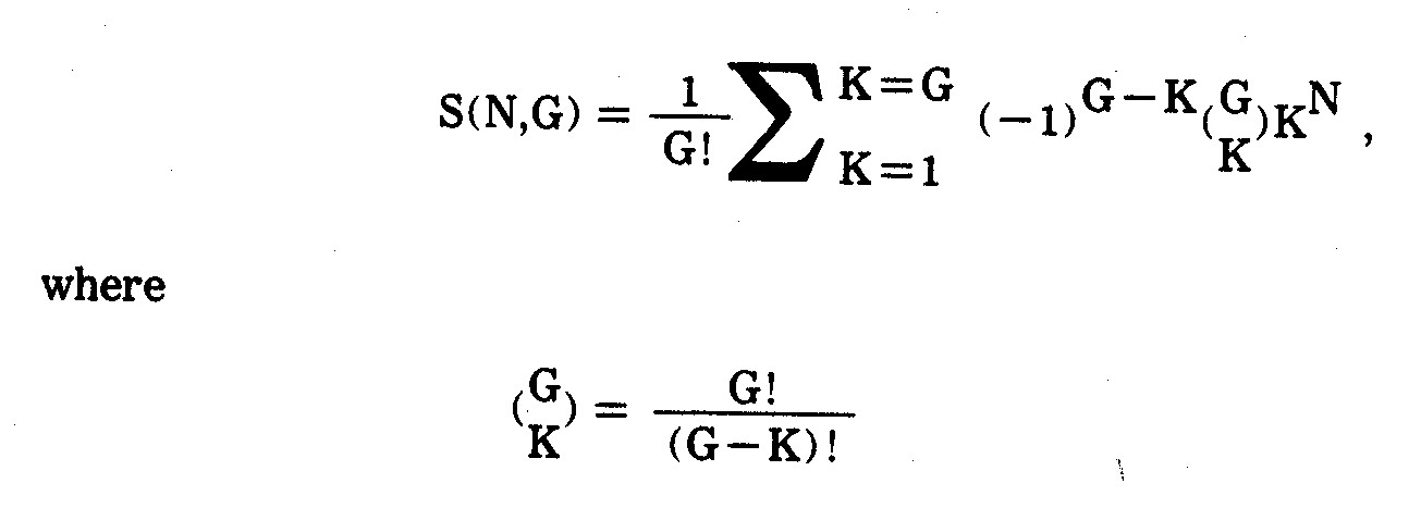
The above S(N,G) formula is known as the
closed-form formula for Stirlings' Numbers of the Second Kind. A serious
problem in both deriving and evaluating clusters is that S(N,G) explodes into
astronomical values for even small N values. An added complication in
cluster analysis is that the nature or number of groups (clusters) to be formed
is not usually specified in advance. Hence, the total number of clustering
outcomes in such circumstances may include all possible numbers of groups
(clusters) from G=1,...,N. As a result, the total number of possible
clustering outcomes becomes an even more astronomical TOTS(N,N) value given by
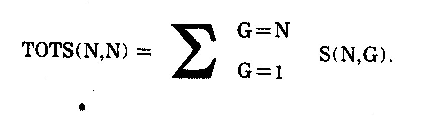
For example, the TOTS(12,12)=4,213,597 number of
feasible ways of partitioning the N=12 electric utility companies into nonempty
and mutually exclusive clusters is derived in Table 6.8. Even in this
"small" clustering problem, total enumeration of all clustering
alternatives is computationally very expensive. Given some type of
clustering homogeneity criterion, however, the cluster analyst would like to
know the "best" clustering alternative for each G value of interest.

Some years back I developed a dynamic programming
algorithm designed to yield the optimal clustering solutions without having to
enumerate all feasible clustering alternatives.51 A number of other
researchers have also formulated integer programming approaches.52 But
neither dynamic programming nor integer programming are sufficiently efficient
for most clustering problems (other than very small or large problems having
special structure). In most instances, a heuristic (hierarchical, linkage)
algorithm must be resorted to, some of which are extremely efficient and
popular.53 A review of various techniques is given by Anderberg, Everitt
and Duran and Odell.54
There are many variations in cluster analysis,
some which are discussed below:
(1) Whether or not entities are directly
traceable to one or more groups. For example, factor analysis, principal
component analysis, and multidimensional scaling can sometimes be viewed as
types of cluster analysis in which items (entities or variates) are
represented by a smaller number of factor, component, or axis groupings
which are composites of the items. However, individual items
(entities) are not sorted and allocated to groupings in such a manner
that any group contains an identifiable subset of specific items (entities).55 Unless noted otherwise, I will usually assume that items
being grouped are directly traceable to one or more groups, as is usually the
case in clustering and classification models.
(2) Whether or not entities are partitioned
into mutually exclusive groups. In most instances, cluster analysis has
been applied where N entities are to be partitioned into both mutually
exclusive and collectively exhaustive groups. However, some applications
exist where groups (clusters) overlap.56 Overlapping groups greatly
complicate the number of clustering alternatives and the analysis and
interpretation of clustering outcomes. Unless noted otherwise, it is
generally assumed implicitly that groups do not overlap, i.e., that
groups are mutually exclusive.
(3) Whether or not pairwise association indices
of similarity (e.g., correlation coefficients) or dissimilarity (e.g.,
Euclidean distances) are utilized in the clustering algorithm. In most
instances such indices between pairs of items are utilized. A number of
clustering algorithms do not, however, require pairwise comparisons using such
indices, e.g., direct clustering methods of Hartigan57 and normix (or mixture)
analysis by Wolfe.58
(4) Whether or not clustering algorithms are
objective or subjective. In most instances, clusters are generated by
"objective" numerical algorithms on a computer. In other
instances, however, display techniques may be used, requiring human observers
subjectively to form the clusters, e.g., clustering by visual comparisons of
profiles and caricatures illustrated previously in this chapter.
(5) Whether or not clusters are
"optimal" in terms of a stated objective function. Many
clustering algorithms are hierarchical in nature such that the number of
groups (clusters) varies from stage to stage of the algorithm. At a
given stage, the partitionings of the entities are not necessarily
"optimal" in terms of the clustering objective function.
Often, however, it is not practical to further attempt to find the optimal
clusters at each stage of the hierarchy.
Hierarchical clustering techniques may be
further subdivided into those which are divisive versus agglomerative. A
divisive hierarchical technique beings with all entities lumped
together and then splits them into smaller and smaller subsets until each
entity comprises a cluster by itself. An agglomerative hierarchical
approach begins with each entity in a separate cluster and then successively
combines (merges) clusters until at the final stage all entities fall into a
single cluster. The analyst then chooses one or more intervening stages
to analyze in greater detail.
(6) Whether entities or variates are to be
clustered. In most instances, entities are clustered on the basis of
variates observed on each of the entities. It is possible, however, to
cluster the variates rather than entities. It is also possible to
cluster both variates and entities at the same time.
(7) Whether or not all variates are measured in
mixed scales. In most instances, variates under study are all
continuous, all ordinal, or all nominal. In a mixed-scale problem some
of the variates may be a combination of continuous, ordinal, and
nominal. Mixed scale problems are difficult to deal with in numerical
approaches, and hence, the analyst may prefer to resort to subjective
approaches.
(8) Whether clusters are to be predictive
rather than merely descriptive. Descriptive clusters are evaluated only
in terms of the internal input variates used in the clustering process.
Predictive clusters are normally evaluated in terms of some external criterion
variate
not used in the clustering process but subsequently of interest after the
clusters are identified.
50 Terms
other than cluster analysis which arise in the literature include clumping,
partitioning, grouping, or classifying theory.
51 Robert E.
Jensen, "A Dynamic Programming Algorithm for Cluster Analysis," The
Journal of Operations Research, Vol. 17, 1969, pp. 1034-57. Also
reproduced in B. S. Duran and P. L. Odell, Cluster Analysis: A Survey
(New York: Springer-Verlag, Chapter 3, 1974).
52 See, for
example, H. D. Vinod, "Integer Programming and the Theory of
Grouping," Journal of the American Statistical Association, June
1969, pp. 506-19. One of the best formulations to date was presented by
George Diehr, "Minimum Variance Partitions and Mathematical
Programming," Paper Presented at the National Meetings of The
Classification Society, Atlanta, Georgia, April 1973.
53 One exceedingly
popular formulation is the hierarchical algorithm described by J. H. Ward,
"Hierarchical Grouping to Optimize an Objective Function," Journal
of the American Statistical Association, Vol. 58, 1963, pp. 236-44. An
even more computationally efficient approach for large N is the k-means
algorithm derived by J. B. MacQueen, "Some Methods of Classification and
Analysis of Multivariate Observations," Proceedings of the Fifth Berkeley
Symposium On Mathematical Statistics and Probability (Berkeley: University
of California Press, 1967, pp. 280-98).
54 M. R.
Anderberg, Cluster Analysis for Applications (New York: Academic Press,
1973). B. Everitt, Cluster Analysis (New York: Halsted Press,
1974). B. S. Duran and P. L. Odell, Cluster Analysis: A Survey (New
York: Springer-Verlag, 1974.)
55 The term
item is used since either entities or variates may be grouped, and in some cases
both entities and variates are grouped. It will be convenient to assume,
however, that items to be grouped are entities (rather than variates) unless
explicitly stated otherwise.
56 Examples
of cluster analysis with overlapping groups include: R. M. Needham, "A
Method for Using Computers in Information Classification," Proceedings of
I.F.I.P. Congress, 1962, p. 284-298; R. M. Needham and K. S. Jones,
"Keyword and Clumps," Journal of Documentation, Vol. 20, 1964,
pp. 5-15; A. G. Dale, N. Dale, and E. D. Pendergraft, "A Programming System
for Automatic Classification With Applications in Linguistic and Information
Retrieval Research," Paper No. LRC64, WTM-5, Linguistics Research Center,
1964; M. G. Kendall, "Discrimination and Classification," in P. R.
Krishnaiah (Editor), Multivariate Analysis (New York: Academic Press,
1966, 165-84); L. L. McQuitty, "Agreement Analysis: Classifying Persons by
Predominant Patterns of Responses," The British J. of Statistical
Psychology, Vol. 9, 1956, pp. 5-16.
57 J. A.
Hartigan, "Direct Clustering of a Data Matrix," Journal of the
American Statistical Association, Vol. 67, 1972, pp. 123-29.
58 J. H.
Wolfe, "NORMIX: Computational Methods for Estimating the Parameters of
Multivariate Mixtures of Distributions," Research Memorandum, SRM
68-2, U.S. Naval Personnel Research Activity, San Diego, 1967; also see
"Pattern Clustering by Multivariate Mixture Analysis," Multivariate
Behavioral Research, Vol. 5, 1970, pp. 329-50.
6.7.5--Euclidean Distances Between Companies.
In earlier sections clusterings of N=12 electric utility companies on the basis
of profile or caricature visual displays were illustrated. A numerical
clustering approach will now be illustrated. The following elements are
utilized:
DATA--Standardized factor scores in Table 6.6:
MEASURES OF ASSOCIATION--Euclidean distances
between pairs of companies;
CLUSTERING ALGORITHM--The JENCLS General
Classification Program at the University of Maine (a clustering routine
comparable to Ward's hierarchical grouping routine mentioned previously.
DENDOGRAPH--A tree-like diagram depicting the
entity (company) mergings into clusters at sequential stages in the
hierarchical clustering algorithm.
The data and Euclidean distances are shown in
Table 6.9. The pair of companies most alike (with Euclidean
distance of 0.38 in terms of the three major factors from Table 6.6) underlying
the ten criteria (from Table 6.2) are Florida Power and Light (FPL) and Northern
States Power (NSP). Their factor score similarities (see Exhibit 6.3) are
somewhat surprising since these two companies exhibit rather large differences
among the M=10 original criteria in Table 6.2. The next closest pair of
companies consists of Commonwealth Edison (COM) and The Southern Company (COM)
with a Euclidean distance of 0.61 in Table 6.10.
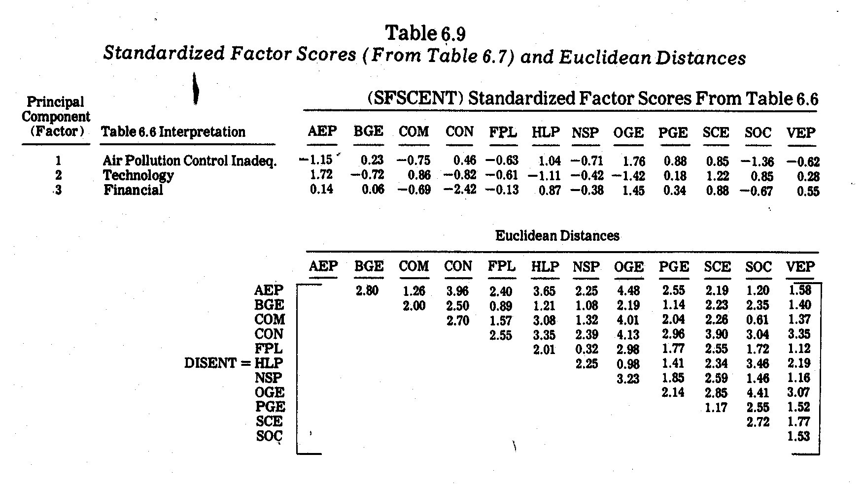
In contrast, American Electric Power (AEP) and
Oklahoma Gas and Electric (OGE) are least alike with a Euclidean distance
of 4.48. This is not surprising since AEP is an immense coal-fired
conglomerate with severe pollution problems but a relatively high R&D
commitment. The OGE company, on the other hand, is a much smaller natural
gas-fired company with almost no particulate and sulphur dioxide emission
problems but higher electricity prices and underinvestment in nitrogen oxides
emission control. The OGE company also has a much lower R&D
expenditure as a proportion of revenues.
Use of standardized scores has an advantage of not
differentially weighting individual variates because of scaling
differences. Use of factor scores (from Table 6.6) in lieu of the M=10
original variates has an added advantage of linear independence (orthogonality)
between inputs in the Euclidean distance calculations. For example, if
Euclidean distances were calculated from the M=10 variates in Table 6.2 (after
variate standardization), correlated pollution or other variates would be
"double counted" and, thereby, tend to overwhelm individual variates
by themselves. Factor analysis recasts the entire system of variates into
fewer "factors" which are not correlated, and hence, are not double
counted in Euclidean distance calculations.
6.7.6--Hierarchical Clustering Outcomes.
Enumeration of all TOTS(12,12)=4,213,597 possible clustering outcomes (see Table
6.9) seemed impractical for this study. Instead an agglomerative
hierarchical approach59 was used in which all N=12 companies
are first viewed as G=12 single-entity clusters at Stage 1. At Stage 2,
the closest pair of companies (in terms of Table 6.9 Euclidean distances) are
merged into one cluster, thereby leaving G=11 clusters at Stage 2. Two
clusters are merged in each succeeding stage until at Stage 12 all N=12
companies are forced into G=1 cluster.
The hierarchical mergings of these electric
utility companies into clusters are pictured in a dendograph-type diagram in
Exhibit 6.8. Unfortunately, there are no statistical tests or generally
accepted mathematical criteria as to what stage (i.e., as to the number, G, of
cluster groupings) should be considered "best." Parsimony
increases as there are fewer and fewer clusters, i.e., as G becomes
smaller. Usually, however, this parsimony is offset by decreasing
within-group homogeneity as entities (in this case electric utility companies)
are forced into larger and larger clusters.
One clustering homogeneity criterion is the
pooled within-groups sums of squares, otherwise known as "Trace W"
criterion,60 where W is the dispersion matrix on all the
variates (in this case the three-factors in Table 6.10). Although the use
of Trace W as a "stopping" criterion is somewhat controversial,61
the Trace W values at each clustering stage are shown in Exhibit 6.8.62
The large jump in Trace W between Stages 8 and 9 suggests that Stage 8 yields
relatively homogeneous clusters and parsimonious groupings of the companies into
G=5 groups (clusters), which might be viewed here as empirical "types"
in terms of the original M=10 social impact criteria in Table 6.2.
The Stage 8 clusterings into "types are as
follows:

Cluster 1 is comprised of the largest coal-fired
companies. Clusters 4 and 5 contain the least-polluting companies with
much higher natural gas usage. Conversely, Clusters 4 versus 5
differ primarily in terms of size and R&D expenditures as a proportion of
revenues (the three underlying major factors on which the Exhibit 6.8
clusterings are based were briefly interpreted in Table 6.5), i.e., Cluster 5
companies have a much higher commitment to R&D than Cluster 4
companies. Consolidated Edison of New York (CON) stands apart (Cluster 3)
from all other companies, in large measure due to its exceptionally poor
performance on Factor 3, i.e., due to having the lowest earnings margin and the
highest kwh prices on electricity of all the companies in the study.
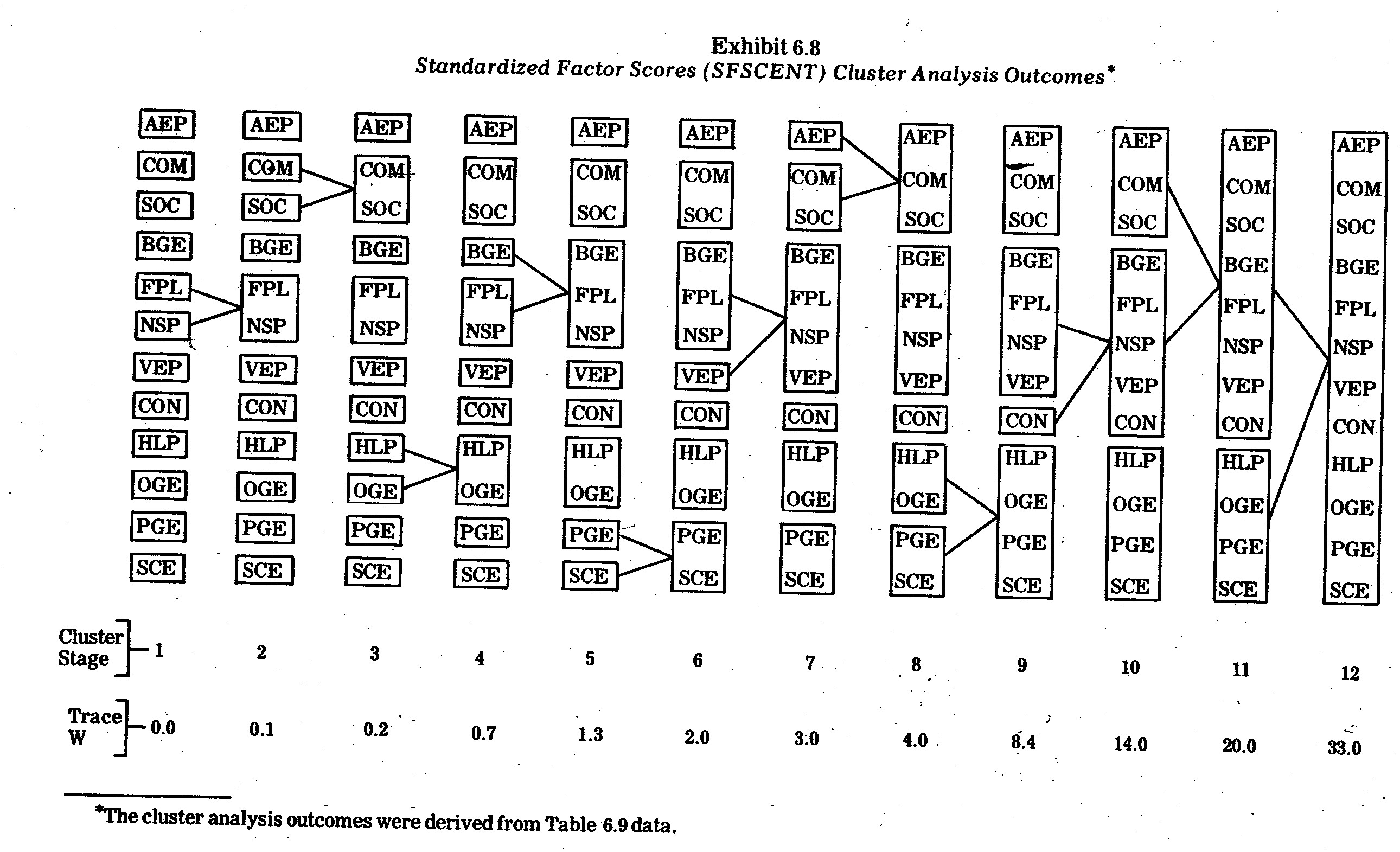
59 My JENCLS
General Classification Program at the University of Maine was utilized.
The program contains a hierarchical clustering algorithm which, for this data,
yields clusterings in a similar manner to Ward's hierarchical grouping program,
i.e., See J. H. Ward, Op. Cit.
60 Other criteria
such as |W| and G|W[ are discussed elsewhere. See, for example, F. H. C.
Marriott, "Practical Problems in a Method of Cluster Analysis," Biometrics,
Vol. 27, 1971 pp. 501-14.
61 See Robert
L. Thorndike, "Who Belongs in the Family?", Psychometrika, Vol.
18, 1953, pp. 267-76.
62 When
Euclidean distances are available it is easier to compute Trace W from averaged
sums of all pairwise Euclidean distances (squared) in the manner described in
Robert E. Jensen, "A Dynamic Programming Algorithm for Cluster
Analysis," Journal of Operations Research, Vol. 17, 1969, pp.
1034-57.
63 These
clustering outcomes are given at Stage 8 in Exhibit 6.8.
6.8--Summary
The major intent of this chapter was to explore
means by which multivariate social criteria can be simultaneously compared on
companies without having to convert everything into monetary units (as is the
case in traditional financial accounting). Graphic and other display
techniques were considered. An important advantage of display techniques
lies in the ability to exploit human mental powers in sorting and making
comparisons between entities and/or variates. Another advantage is the
ability to combine both quantitative and qualitative variations in a single
display.
Drawbacks of visual displays lie mainly in the
subjectivity and obvious cumbersomeness of making comparisons if many entities
and/or considerable detail are included in the display. Profile charts,
for example, are highly satisfactory where there are small numbers (e.g., less
than twelve) of entities and a few (e.g., less than six) quantitative
variates. Certain mathematical transformations (e.g., principal component
analysis) may help to reduce the number of variates to be treated in the
display, although interpretations may be somewhat complex. Fourier series
plots appear to have few advantages over profile plots except where there are
too many variates (or factors) for profile plots. Also statistical
inference testing becomes possible when a number of restrictive assumptions are
satisfied in the Fourier series model.
Geometric pattern and/or caricature displays may
accommodate more entities and variates than do profile charts. In
addition, qualitative variations may be accommodated in many types of such
displays. Two such approaches illustrated in this chapter were glyph plots
and facial caricatures. Facial caricatures can be utilized for a greater
number of variates than can glyphs, although the facial comparisons become quite
dependent upon how human viewers subjectively weight different features when
comparing faces. There will also be skeptics who view comparisons of
abstract representations (such as faces) as being nonsense or silly
fun-and-games.
Cluster analysis and other tools in numerical
taxonomy were designed primarily to overcome some of the difficulties caused by
subjectivity in taxonomy classifications in the natural sciences.
Numerical techniques have the important advantage of yielding
"objective" groupings (provided the variates and appropriate
mathematical approaches can be agreed upon) in the sense that allocations of
entities (or variates) to groups is accomplished by mathematical techniques
(usually on a computer) rather than human observers. This advantage,
however, is offset by computational difficulties and the fact that different
approaches work better than others for certain types of clusterings. In
contrast, the human mind is much more flexible (e.g., when presented with visual
displays) in detecting clusters and abberrations.
In practice it is probably best to compare
"subjective" visual display clusterings with "objective"
numerical clusterings. Both approaches were illustrated in this
chapter. For example, Table 6.2 listed performance data for N=12 private
electric utility companies on M=10 social impact criteria. A principal
component analysis was performed, reducing these criteria to three underlying
independent factors (interpreted in Table 6.5). Rotated factor scores were
then analyzed in visual displays (profile charts and facial caricatures) and in
a hierarchical clustering algorithm. Although the number of clusters which
emerge is open to debate, it seemed to me that Stage 8 was a reasonable stopping
point (where G=5 clusters) in Exhibit 6.8. The human observers I presented
with the Exhibit 6.7 faces tended to choose G=4 clusters. The groupings in
both cases were similar but not identical, as is indicated in Exhibit 6.9.
In particular, the BGE classification seems to be the least consistent.
The "objective" numerical clusterings in Exhibit 6.8 include BGE with
CEP, FPL, and NSP. This is consistent with their Factor 2 (Technology) and
Factor 3 (Financial) similarities evidenced in Exhibit 6.3. However,
Exhibit 6.3 also reveals how BGE (and CON) pull ahead of the pack with respect
to Factor 1 (State-of-the-Art Pollution Control). This is especially
surprising since BGE is a relatively heavy coal user (59.1% under x2
in Table 6.2). The exceptional performance (relative to other coal and/or
oil burning companies) on particulate and sulphur dioxide control seems to be
the reason for BGE's inclusion with the "clean guys" in Cluster 4 in
Exhibit 6.7. But the falling down of BGE on Factors 2 and 3 (see Exhibit
6.3), however, partly explains the inconsistencies in BGE classifications in
Exhibit 6.7 versus Exhibit 6.8. Similarly, the exceptional Factor 1
performance of CON also gives it certain facial features resembling Cluster 4
"clean guys" in Exhibit 6.7.
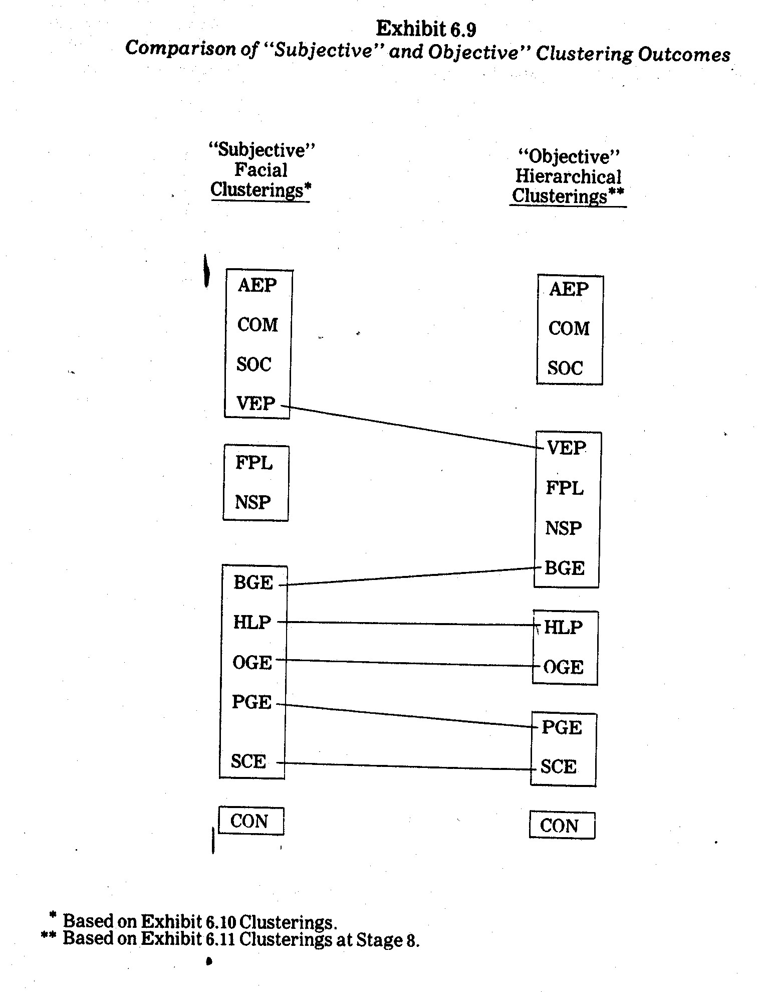
As expected, the "objective"
hierarchical clusterings in Exhibit 6.8 (based on Euclidean distances) agree
more closely with profile similarities in Exhibit 6.3 than do the
"subjective" clusterings in Exhibit 6.7. The
"subjective" facial clusterings differ largely because of apparent
unequal weightings given to different facial features by human observers.
For example, eyebrow size and shape variations seem to be much less important
than eye size and shape variations. One means of overcoming this problem
is to make a number of facial plottings under different assignments of variates
(or factors) to facial features and attempt to discover if human observers tend
to detect consistent clusters under such variations.
I stress that no significance whatever should be
placed upon which companies have the most "agreeable,"
"appealing," or "happy" faces. In both Exhibits 6.6
and 6.7, the social impact variates (or factors) were randomly assigned to
facial features. The purpose is merely to compare faces with one another
in an effort to discover subsets which seem to be most (or least) alike.
One advantage of the caricature (e.g., glyphs or faces) comparisons (e.g., see
Exhibit 6.7) relative to numerical clustering outcomes (see Exhibit 6.8) is that
alternative clusterings are a little more evident. For example, in Exhibit
6.7 it is evident that, although BGE has certain things in common with most
other Cluster 4 companies (e.g., head size, head shape, nose length, mouth
length, position of center of mouth, separation between centers of eyes, and
position of pupils), BGE also has features in common with CON in Cluster 1
(e.g., eyebrow length, height of centers of eyes, half-length of eyes, and angle
of brows). This similarity is also evident in the profiles in Exhibit 6.3
but is not shown as clearly in the cluster-merging (dendograph) diagram in
Exhibit 6.8.
Both "objective" and
"subjective" cluster analysis approaches illustrated in this chapter
are means by which entities (e.g., companies) may be sorted into
"types" on the basis of multivariate criteria (e.g., the M=10 social
impact criteria in Table 6.2). The interpretation of these
"types," and more particularly the ranking of the "types"
along a "good versus bad" or "high versus low"
composite of all criteria simultaneously, is a much more difficult and
controversial undertaking. Material in Chapters 7 and 8 have some
relevance to such endeavors.
6.9--Suggestions for Further Research
The number of criteria (i.e., the M=10 variates
in Table 6.2) is too small for a thorough taxonomy study of corporate social
criteria. Many additional criteria (e.g., see Appendix A ) must be
considered. However, relevant data on which corporations can be compared
along a much wider spectrum are lacking. It seems that future corporate
comparisons such as those illustrated in this chapter will await better
data. Such data might either be generated in large-scale studies of
companies or from required (and uniform) reporting practices imposed upon
corporations. Internal studies by the companies themselves are of less use due to
likely inconsistencies in definitions, measurement techniques, accuracy, and
scope of investigation.
Much further study is obviously needed to
determine what attributes (criteria) are most important to study. The
added Chapter 5 considerations must be better resolved. If data become
available, however, multivariate analyses such as those mentioned in this
chapter are especially interesting to pursue, e.g., in both seeking underlying
factors amidst criteria and empirical "types" of companies.
Dimensions of social conflict and interaction are also of interest in future
research. Chapter 7, in particular, bears upon such issues.
Clusterings in this chapter concerned companies
at a point in time. Another area of interest might be the study of
evolutionary patterns over time with respect to economic, social, and
environmental criteria. For example, cladistic taxonomy64
reconstructs the branching patterns over different time planes. This might
be further extended to considerations of evolutionary rates, parallelism, and
convergence.
64
Classification by clades is discussed in J. S. Huxley, "Evolutionary
Processes and Taxonomy With Special Reference to Grades," Uppsala
University Arssks, 1958, pp. 21-39. For other references, see Chapter 6
in P. H. A. Sneath and R. R. Sokal, Numerical Taxonomy (San Francisco: W.
H. Freeman and Company, 1973).
|
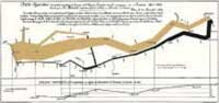
http://www.cs.trinity.edu/~rjensen/MicrosoftInv
Your students may also want to learn how to prepare their own pivot tables and pivot charts.
Go to the ExcelPivotTable01.wmv video listed at http://www.cs.trinity.edu/~rjensen/video/acct5342/
Bob Jensen
http://faculty.trinity.edu/rjensen/